9.1.1 Virtualization, containers, orchestration
The usual teaching sequence for this domain, and a reasonable order to learn it in:
- Virtualization — concepts and types
- Containers — VMs vs containers, Docker
- Orchestration — scheduling, service discovery, rolling updates; in practice Kubernetes
- Non-functional capabilities of the resulting platform
Three implementations of virtualization differ by how they intercept the guest OS: full (software-emulation) virtualization, where the hypervisor traps and emulates every privileged instruction so the guest OS runs unmodified; paravirtualization, where the guest OS is itself modified to cooperate with the hypervisor via hypercalls instead of trapped instructions, trading portability for lower overhead; and hardware-assisted virtualization, where CPU extensions such as Intel VT-x and AMD-V let the hypervisor run guest instructions natively. This last variant is what made virtualization efficient enough to become the cloud's substrate.
A virtual machine is a software emulation of a computer that runs in an isolated partition of a real machine, complete with its own guest operating system, whereas a container is essentially a sandbox for a single process that shares the host kernel instead of emulating hardware — the reason containers start and stop in a fraction of a second while VMs must boot a full OS. Docker itself resists a one-line definition: it functions at once as an image format, a container runtime, an image-build system, a remote management API, a log-collection daemon, and an orchestrator, which is why practitioners often reduce it to "a wonderful mechanism for shipping tarballs."
Containers share one host OS and kernel; each VM duplicates a full guest OS — the source of both the VM's stronger isolation and its slower startup.
9.1.2 Cloud core
The NIST definition
The NIST definition of cloud computing has been the most accepted and is used as the basic definition. A simplified version: remote computing resources provided as a service. By computing resources we usually mean network, computing units (virtual machines), and storage.
The NIST definition introduces five fundamental properties that characterize a cloud offering:
| Property | Meaning |
|---|---|
| On-demand self-service | A consumer can unilaterally provision computing capabilities |
| Broad network access | Capabilities are available over the network and accessed through standard mechanisms that promote use by heterogeneous thin or thick client platforms |
| Resource pooling | The provider's computing resources are pooled to serve multiple consumers using a multi-tenant model, with different physical and virtual resources dynamically assigned and reassigned according to consumer demand |
| Rapid elasticity | Capabilities can be elastically provisioned and released, in some cases automatically |
| Measured service | Resource usage can be monitored, controlled and reported, providing transparency for both the provider and the consumer |
Automated elasticity matters because the actual demand is often not what we can predict — automated elasticity provided by cloud can be far more beneficial than managing scale manually.
Cloud types: public, private, hybrid — and also a community cloud.
OpenStack is an open-source cloud operating system and community founded by Rackspace and NASA in 2010. It is an abstraction over the hypervisor and provides a unified interface to access the various resources — compute, storage (object and block), and network.
Service models
Security and compliance is normally a shared responsibility between the cloud provider and its customers — for example, the AWS Shared Responsibility Model describes such segregation.
| Model | Definition |
|---|---|
| IaaS | Gartner: a standardized, highly automated offering where compute resources, complemented by storage and networking capabilities, are owned by a service provider and offered to the customer on demand. The resources are scalable and elastic in near real time and metered by use. Self-service interfaces are exposed directly to the customer, including a web-based UI and an API. The resources may be single-tenant or multitenant, and hosted by the service provider or on-premises in the customer's data center — the public/private cloud distinction |
| PaaS | Platform services. In recent years Gartner combines IaaS and PaaS providers into one quadrant |
| hpaPaaS | Gartner defines a special subset of PaaS: high-productivity application platform as a service. These provide services for declarative, model-driven application design and development, and simplified one-button deployments. They typically create metadata and interpret it at runtime; many allow optional procedural programming extensions. The underlying infrastructure is opaque to the user — they do not deal with servers or containers directly. The rapid application development features are often referred to as "low code" and "no code" support. hpaPaaS solutions provide: UI capabilities via responsive web and mobile apps; orchestration or choreography of pages, business processes, and decisions or business rules; a built-in database; and one-button deployment |
| SaaS | One of the main architectural problems to solve is tenant isolation — on different layers — for multi-tenant systems |
| Serverless | Presented via the Serverless Compute Manifesto, and compared side by side against VMs and containers |
Cloud service taxonomy
IaaS services
| Group | Services covered |
|---|---|
| Networking | Virtual networks; internet gateway; network ACLs; security groups; load balancing; DNS; CDN |
| Storage | File & block storage; object storage; performance tiers; Azure Storage specifics |
| Compute | Instance characteristics; instance types; compute features |
PaaS services
| Group | Services covered |
|---|---|
| Application | aPaaS; API management; queues |
| Database | Relational databases; NoSQL; cache |
| Analytics | Not considered in the course |
On API management vs an API gateway — the distinction matters:
API management allows you to know the answers to questions like: who are your top developers? Are you attracting more developers? Do you know how your API traffic is trending over time? It also provides management for the entire lifecycle of the API and tools for all stakeholders — whereas an API gateway is limited to exposing information to handle requests and services.
Architecting for the cloud
Disposable resources and immutable infrastructure
With fully automated deployment methods you can replace old components with new versions to ensure your systems maintain their initial "known-good" state. Managing a fleet of instances becomes much simpler with immutable infrastructure, since there's no need to track the changes that would occur.
With immutable infrastructure you know what's running and how it behaves. Deploying updates can become routine and continuous, with fewer failures occurring in production, and all changes are tracked by your source control and CI/CD processes.
The four rules:
| Rule | Rationale |
|---|---|
| Don't modify instances in place | This is the core pattern in immutable infrastructure. Modifying server instances is difficult to successfully automate and track, and allowing it will result in manual modifications. While in theory it is possible to have policies and tools in place to keep things consistent, in practice both fail with some regularity. There is no concise and trustworthy way to know if and where you have configuration drift |
| Replace instances to update them | If nothing is changed in situ, then to introduce change we must be able to deploy new instances without affecting the customer experience. While this can be done manually it rarely works well, as humans are bad at following rote procedures consistently. Plan to automate instance replacement |
| Plan for instance and zone failures at all times | Instance failure should be a normal part of doing business — whether unintended due to bugs or other issues, or intentional in order to perform component replacements. Zone failures on AWS and Google Cloud should also be relatively painless if you architect well; on Azure you'll want to use Availability Sets |
| Don't let instances get stale | Not unlike a computer, the longer an instance has been in use, the greater the chance it will have drifted from the optimal configuration. Don't run server instances for a long time |
Pets vs cattle: are you operating in the type of environment that, if one server crashes, everything goes down — a "Pet" — or are you in a scenario in which the loss of a server means that nothing happens, because the "herd" still exists and performs just as before — "Cattle"?
Availability itself has a computable definition worth carrying into an ASR. For components chained with no redundancy, overall availability is the product of each component's availability — e.g. 99.5% × 99.9% × 99.9% ≈ 99.4%, so single points of failure compound quickly. For components deployed redundantly in parallel, availability instead becomes A₁ + (1 − A₁) × A₂ — e.g. two components each at 99.5% combine to roughly 99.9975% — the quantitative case for why redundancy, not just component quality, is what buys the "nines" of uptime. This is also why zone failures need a redundancy plan rather than hoping a single Availability Set is enough.
Automation
As failures are expected and accepted, we should design our architecture with this in mind. In order to recover quickly from a failure we have to react quickly. Another motivation to move fast in the cloud is to be able to respond quickly to any new requirement or change in the market. Fortunately several tools and strategies support these notions:
| Capability | Meaning |
|---|---|
| Auto recovery | When something goes down it should be noticed and recreated in an automated way |
| Auto scaling | Automatically scale up or down to the actual load and calling pattern |
| Observability | Our system must be fully interrogable at every time — observability is a very fundamental requirement |
| Easy experimentation | To support faster time-to-market and respond to market changes quickly, we should make experimentation easier — using frameworks that allow quick application development and deployment while meeting the requirements above |
When the destination is decided, the move itself is usually planned against the 6 Rs of cloud migration: retain (keep it on-premises, revisit later), rehost (lift-and-shift onto IaaS with minimal effort), replatform (some application changes, such as moving the database to a hosted DB service), refactor (middleware or application changes to consume PaaS), replace (architectural changes and porting to a SaaS offering), and retire (decommission the application and its host, migrating nothing). Which R applies to a given application is itself an architectural call, driven by financial, security, business, technical, and compliance assessments of that specific workload.
Cascading failures
In interservice communication, one slow application instance without proper isolation can easily slow down the entire system.
The course's memorable analogy: a mailing list where somebody asked something; after a point most people weren't interested in the discussion, and somebody sent an unsubscribe request to the list — everybody started to do the same, creating a huge message flood and making the situation more serious.
Many different techniques help here — see the bulkhead and circuit breaker patterns in Module 4.
Loose coupling and application-level resilience
Interservice communication should be isolated, and resilience is implemented at the application level with a specific toolkit: bulkheading, proper timeouts — timeout deadlines matter — circuit breaking, and async libraries. These are the Module 4 patterns arriving as cloud operational necessities rather than optional refinements.
Cloud Native — and what it is not
Cloud Native is a commonly misunderstood term. The point is that Cloud Native is not about cloud and leveraging the cloud.
The term refers to software built for change, scale, resilience and manageability. It is often equated with microservices and containers, but those aren't required. Whether running in public or private clouds, a cloud-native app takes advantage of the elasticity and automation offered by the host platform.
The cloud-native approach is far more about "how" than it is about "where."
The right question is: what capabilities and practices make it economical to work in small batches, test hypotheses, and learn? The answer is capabilities like cheap application builds, safe deployments, automated management of deployments (start/stop/scale/health checking), security, distributed configuration, and traffic routing. Containers play a foundational role in implementing these capabilities and form the basis of the platforms that provide them — but the capabilities are what are important, not the containers.
The 12-factor principles that matter most here
The 12-factor methodology provides factors applicable in any language to software delivered as a service. Three of them carry most of the weight for cloud design:
| Principle | Why it matters |
|---|---|
| Stateless and share-nothing processes | Data — whether for state or other reasons — limits the ability to distribute or easily scale a process. Never design a process that expects a set of data to be persisted locally. All data should be persisted outside the process using an attached service |
| Dependencies explicitly declared and isolated | In practice this means the application is environment agnostic and doesn't expect some tool or library to exist outside what is explicitly declared |
| Config distinct from code | Anything distinct to an execution environment — development versus production credentials, connection strings, unique hostnames — stored in a config file separate from the code that uses it |
Why containers, specifically
Containers are increasingly popular because once an application is containerised it is easy to package, ship, and run anywhere. Unlike traditional virtualization, containers provide lightweight virtualization at the application level, and are therefore much better at squeezing every last ounce of available capacity.
The operationally decisive property: containers can start and stop at sub-second speeds, which makes it easy both to scale out and to recover from failures — simply by starting up new containers.
9.2 Web and Mobile
Choosing a web platform
Platform choice is best framed as a decision tree, and these are the questions worth asking:
| If the requirement is… | The answer tends to be |
|---|---|
| Just a simple website with static HTML pages, fast page configuration and customisation | Static site generators — Hugo, Jekyll, Gatsby |
| Content managed centrally but delivered to multiple client channels / different web apps | Headless CMS — Strapi, Contentful, Drupal headless |
| A conventional content-managed site | Traditional CMS — WordPress, Drupal, Joomla |
| Behaviour driven by configuration files and a custom configuration system | Dynamic websites with a custom configuration system |
Two selection criteria the course calls out explicitly, because they are architectural rather than cosmetic:
- Why security matters in the choice. Different site builders and CMS platforms provide different levels of security out of the box. Drupal has over the years earned a reputation for secure and robust performance; this is not so positive for WordPress, which attracts far more security threats and malware attacks
- Why performance matters in the choice. Different builders are built on platforms and frameworks with different performance characteristics. Some provide optimisation techniques out of the box — GZIP compression, caching. And simple static site generators are much faster than the alternatives
Micro frontends
The micro frontends approach is a great technique to divide the workload in a multi-team setup and isolate code.
The trigger condition is a frontend that has become too big to be supported as one unit, or teams that must ship independently. It is the Module 4 microservices argument — Conway's Law included — applied above the API boundary rather than below it. Fowler's article is the reference.
Choosing a mobile approach
| Approach | Definition | Fits when |
|---|---|---|
| Native | A mobile application created for one platform | Games, graphical apps, apps needing deep device capability |
| Cross-platform | The same codebase adapted to run on different platforms | Broad reach with shared logic |
| PWA | A progressive web application which has an icon on the mobile desktop and can provide other device-like capabilities | Only mobile web reach needed |
| Hybrid | An application that runs as a web application and can be wrapped as a native one | Reuse of web assets with store distribution |
SEO as an architectural concern
SEO means the process of optimising a web application so search engines can display it at the top of search results. For private application parts — e.g. the admin section — SEO should not be available.
That second sentence is the architectural instruction: indexability is a per-area decision, not a site-wide one, and private areas must be excluded deliberately.
The web performance metrics worth putting into a performance ASR for a front end: First Contentful Paint · Speed Index · Time to Interactive · First Meaningful Paint · First CPU Idle · Max Potential First Input Delay · Critical Rendering Path Length.
A second, complementary model worth knowing by name is Google's RAIL model, which frames performance around four user-facing phases rather than page-load timings alone: Response (react to input within 100ms), Animation (each frame completes within 16ms), Idle (non-critical work chunked to fit inside 50ms idle windows so it never blocks input), and Load (meaningful content within roughly 1 second). Where the load metrics above describe a single startup event, RAIL describes the steady-state responsiveness a user experiences throughout a session.
9.3 Cache
High availability for a cache means the ability to continue operating despite the failure of members of the cluster. Applied to distributed caching, HA means uninterrupted, consistent data access. That uninterrupted access is a function of cache topology, not just clustering. An embedded (in-process) cache lives inside the application's own JVM — on-heap, bounded by that JVM's memory, or off-heap, bounded by the server's RAM — and gives the lowest latency but no sharing across instances; a distributed cache runs as its own cluster reachable by many application nodes, and within it data is either replicated (every node holds a full copy, so reads stay local but every write fans out everywhere) or partitioned (each entry lives on one primary node plus backups, trading a network hop for far greater aggregate capacity).
Distributed caches that provide this HA guarantee are commonly implemented as In-Memory Data Grids (IMDGs) — products such as Hazelcast, Oracle Coherence, GigaSpaces XAP and Terracotta fall into this category. Beyond plain key-value storage, mature IMDGs add transactional ACID support, typically via a two-phase commit (2PC) protocol, and rely on concurrency mechanisms such as MVCC (multi-version concurrency control) to keep locking overhead low while still guaranteeing consistency across the cluster.
Eviction algorithms
The choice of eviction policy is an architectural decision driven by the access pattern, and getting it backwards is a classic mistake. Eviction is not the only way an entry leaves the cache: time-to-live (TTL) expires it a fixed duration after it was written regardless of use, while time-to-idle (TTI) expires it after a period with no access; the two settings are independent and are normally combined with an eviction algorithm rather than substituted for one.
| Algorithm | Behaviour | Cost and best fit |
|---|---|---|
| LRU — Least Recently Used | Discards the least recently used items first | Requires keeping track of what was used when, which is expensive if you must guarantee the truly least-recently-used item is discarded. Implementations keep "age bits" per cache line, and every time a cache line is used the age of all other cache lines changes. LRU is actually a family — members include 2Q (Johnson and Shasha) and LRU/K (O'Neil, O'Neil and Weikum) |
| LFU — Least Frequently Used | Counts how often an item is needed; those used least often are discarded | Suits stable popularity distributions |
| MRU — Most Recently Used | Discards, in contrast to LRU, the most recently used items first | Chou and DeWitt (11th VLDB conference): "When a file is being repeatedly scanned in a Looping Sequential reference pattern, MRU is the best replacement algorithm." Later researchers (22nd VLDB) noted that for random access patterns and repeated scans over large datasets — cyclic access patterns — MRU has more hits than LRU because of its tendency to retain older data. Most useful where the older an item is, the more likely it is to be accessed |
| Random replacement | Randomly selects a candidate item and discards it when space is needed | Requires keeping no information about access history at all. For its simplicity it has been used in ARM processors |
The MRU result is the one worth remembering, because it is counter-intuitive: under a looping sequential scan, LRU evicts exactly the pages you are about to need again, and MRU wins. Cache policy must follow the access pattern, not habit.
Eviction policy is only one lever; the other is how the cache stays synchronised with the system of record, which splits into synchronous and asynchronous persistence integration. Synchronously, read-through and write-through route every read or write through the cache so the client only ever talks to the cache; asynchronously, write-behind queues writes and flushes them later for lower write latency, while refresh-ahead proactively repopulates an entry before it would expire.
Read-through and write-through both put the cache in front of the client — the application never talks to storage directly.
9.4 Data, AI and ML
Big data characteristics
| V | Meaning |
|---|---|
| Volume | With every year, the meaning of what big data is changes |
| Variety | Digitally sourced data has variety in that it is collected with varying degrees of structure. Data can be heavily unstructured — audio, video and social media posts. A company can gather more structured data on customers' clicks on its website, or a person can track heart rate and physical activity with a wearable — but data must then be organized in order to be useful. Multi-structured data can involve combinations of structured and unstructured data, organized by similar attributes |
| Velocity | Increasingly, businesses have stringent requirements from the time data is generated to the time actionable insights are delivered to users. Therefore data needs to be collected, stored, processed and analyzed within relatively short windows — ranging from daily to real-time |
Major cloud providers enable processing of huge volumes of data on demand, and every year data processing frameworks are updated and capabilities added.
Using an RDBMS for huge volumes is not recommended — but there are plenty of cases where it was done. One documented case scaled PostgreSQL to 1.2bn records per month.
Data forms
In order to work efficiently with data we have to understand data content.
| Form | Characteristics |
|---|---|
| Structured | Highly organized information that uploads neatly into a relational database — think traditional row database structures — lives in fixed fields, and is easily detectable via search operations or algorithms. Relatively simple to enter, store, query and analyze, but it must be strictly defined in terms of field name and type (alpha, numeric, date, currency), and as a result is often restricted by character numbers or specific terminology. Analysts typically use SQL |
| Unstructured | May have its own internal structure but does not conform neatly into a spreadsheet or database. While unruly in nature it is also incredibly valuable and increasingly available in the form of complex sources: web logs, images, video, email, customer service interactions, sales automation, social media. Most business interactions, in fact, are unstructured in nature. The fundamental challenge is that these sources are difficult for non-technical business users and data analysts alike to unbox, understand and prepare for analytic use. Beyond structure there is the sheer volume — because of this, current data mining techniques often leave out valuable information and make analyzing unstructured data laborious and expensive |
| Semi-structured | Maintains internal tags and markings that identify separate data elements, which enables information grouping and hierarchies. Both documents and databases can be semi-structured. This type represents only about 5–10% of the structured/semi-structured/unstructured data pie, but has critical business usage cases |
File formats
Multiple storage formats are suitable for HDFS — plain text, rich formats like Avro and Parquet, Hadoop-specific formats like sequence files — each with pros and cons depending on use case. Classify them into two simple categories: raw data formats and processed data formats.
The access patterns differ, and so the formats should differ. For processing raw data we usually use all the fields, so the underlying storage must support that efficiently. But we access only a few columns of processed data in analytical queries, so the storage should handle that in the most efficient way in terms of disk I/O.
Raw data formats
| Format | Notes |
|---|---|
| Plain text file | A very common Hadoop use case is storing log files or other plain text files with unstructured data. These text files could easily eat up whole disk space, so proper compression is required depending on use case |
| Structured text data | More sophisticated text files having data in a standardized form — CSV, TSV, XML or JSON |
| Binary files | Images, videos stored as-is |
| Avro | Language-neutral data serialization. Avro-formatted data can be described through a language-independent schema, so it can be shared across applications using different languages. Avro stores the schema in the header of the file, so data is self-describing. Avro files are splittable and compressible, making it a good candidate for Hadoop storage. Schema evolution — the schema used to read an Avro file need not be the same as the schema used to write it, making it possible to add new fields. The schema is usually written in JSON, and can be generated from Java POJOs using Avro-provided utilities |
Processed data formats
| Format | Notes |
|---|---|
| Columnar formats (general) | They eliminate I/O for columns that are not part of the query, so they work well for queries requiring only a subset of columns. They provide better compression because similar data is grouped together |
| Parquet | A columnar format. Well suited for data warehouse kind of solutions where aggregations are required on certain columns over a huge set of data. Provides very good compression — up to 75% when used with compression formats like snappy. Can be read and written using the Avro API and Avro Schema. Also provides predicate pushdown, further reducing disk I/O cost |
| ORC | The other columnar option named |
Columnar vs row formats — Parquet vs Avro. Columnar formats are generally used where you need to query only a few columns rather than all the fields in a row, because their column-oriented storage pattern suits that. Row formats are used where you need to access all the fields of a row. So generally Avro is used to store the raw data, because during processing usually all the fields are required.
Compression. Big data solutions should process large amounts of data in quick time. Compressing data speeds up I/O operations and saves storage space — but this could increase processing time and CPU utilization because of decompression. So balance is required: more compression means smaller data size but more processing and CPU utilization.
Compressed files should also be splittable to support parallel processing. If a file is not splittable it means we cannot input it to multiple tasks running in parallel — and hence we lose the biggest advantage of parallel processing frameworks.
From data to insight
| Level | Definition |
|---|---|
| Data | The representation of facts as text, numbers, graphics, images, sound or video. Technically data is the plural of the Latin datum meaning "a fact", though people commonly use the term as singular. Facts are captured, stored and expressed as data. Data is the raw material we interpret as data consumers to continually create information. Data is always right |
| Information | Data that has been "cleaned" of errors and further processed in a way that makes it easier to measure, visualize and analyze for a specific purpose. Depending on that purpose, processing can involve different operations — combining different sets of data (aggregation), ensuring the collected data is relevant and accurate (validation). For example, we can organize data in a way that exposes relationships between seemingly disparate and disconnected data points. By asking relevant questions about who, what, when and where, we derive valuable information. Information can be wrong |
| Knowledge | Information becomes knowledge when we get to the question of how. When we don't just view information as a description of collected facts but also understand how to apply it to achieve our goals, we turn it into knowledge. This knowledge is often the edge that enterprises have over their competitors |
| Insight | As we uncover relationships that are not explicitly stated as information, we get deeper insights. Applying data science allows us to derive historical, predictive or prescriptive insights, answering "Why did it happen?", "What is likely to happen?", "What should we do to make things happen?" |
While traditional analytics allows us to look backward and discover patterns that happened in the past, modern predictive analytics and machine learning techniques allow us to create a forward-looking ("windshield") view.
Analytics maturity
| Stage | Question | Techniques and characteristics |
|---|---|---|
| Descriptive | What happened | Analyze and summarize historical data; observed customer behaviour; non-traditional data sources such as web crawling and social listening |
| Diagnostic | Why did it happen | Identify the cause of trends and outcomes; observed customer behaviour; the same non-traditional sources |
| Predictive | What could or will happen | Predict outcomes based on the past; forward-looking view of current and future customer view; sentiment scoring; graph analysis and NLP to identify hidden relationships; dual-objective models; behavioural economics |
| Prescriptive | What should we do | Recommend right or optimal actions or decisions; real-time product and service propositions; rapid evaluation of multiple what-if scenarios; optimization of decisions or actions |
| Cognitive | How can we adapt to change | Monitor, decide and act autonomously or semi-autonomously; monitor results on a continuous basis; dynamically adapt based on changing environment and improved predictions; agent-based and dynamic simulation models |
Big data solution requirements
Scalability. The solution must be scalable — but how scalable, and to which capacity? This question can be answered by dividing data and applications into categories, creating a predictive model of capacity needs for each category based on expected growth, and aggregating the results.
Scalability is not just about the size of storage; it has wider implications. The throughput and the speed of access must be scalable. In addition, the system should be able to scale operationally — that is, to grow quite large without a huge increase in dedicated staff.
Self healing. A well-designed big data solution must accommodate component failures and heal itself without human intervention.
Hadoop
| Component | Role |
|---|---|
| Hadoop Commons | Libraries and utilities used by other Hadoop modules |
| Hadoop Clients | Libraries and utilities used to access Hadoop's components |
| HDFS — Hadoop Distributed File System | A scalable system that stores data across multiple machines without prior organization |
| YARN — Yet Another Resource Negotiator | Resource management framework for scheduling and handling resource requests from distributed apps |
| MapReduce | Software programming model for processing large sets of data in parallel; in fact a distributed application on top of YARN |
MapReduce
MapReduce architecture consists mainly of two processing stages — the map stage and the reduce stage — with an intermediate process between them doing shuffle and sorting of the mapper output. The actual MR process happens in the task tracker, and the intermediate data is stored in the local file system.
Mapper phase. The input data splits into two components, Key and Value. The key is writable and comparable in the processing stage; the value is writable only. When a client submits input data, the job tracker assigns tasks to task trackers, and the input data gets split into several input splits — which are logical in nature. A record reader converts these splits into key-value pairs; this is the actual input data format for further processing inside the task tracker. The input format type varies from one application to another, so the programmer has to observe the input data and code accordingly. With Text input format, the key is the byte offset and the value is the entire line. Partition and combiner logic come into map coding logic only to perform special data operations. Data localization occurs only in mapper nodes.
Combiner is also called a mini reducer — the reducer code is placed in the mapper as a combiner. When mapper output is a huge amount of data it requires high network bandwidth; to solve this the reduced code is placed in the mapper as combiner for better performance. The default partition used is Hash partition.
Partitioner. A partition module plays a very important role in partitioning the data received from either different mappers or combiners. It reduces the pressure that builds on the reducer and gives more performance. A customized partition can be performed on any relevant data on a different basis or conditions. It has static and dynamic partitions, which play a very important role in Hadoop as well as Hive. The partitioner splits the data into a number of folders using reducers at the end of the map reduce phase, and runs between mapper and reducer. It is very efficient for query purposes.
Intermediate process. The mapper output undergoes shuffle and sorting. The intermediate data is stored in the local file system without having replications in Hadoop nodes. This is data generated after computations based on certain logic. Hadoop uses a Round-Robin algorithm to write the intermediate data to local disk.
Reducer phase. Shuffled and sorted data passes as input to the reducer. In this phase all incoming data combines and the same actual key-value pairs get written into HDFS; a record writer writes data from reducer to HDFS. The reducer is not mandatory for searching and mapping purposes. Options are provided to set the number of reducers for each job — in mapred-site.xml you set properties enabling the number of reducers for a particular task.
Speculative execution plays an important role during job processing: if two or more mappers are working on the same data and one mapper is running slow, the job tracker assigns tasks to the next mapper to run the program fast. The execution is FIFO.
YARN
Individual machines are known as nodes; a cluster can have as few as one node or as many as several thousand. There are two types of node — ResourceManager (RM) and NodeManager (NM).
ResourceManager manages the cluster resources.
- A cluster can have only one RM — but it is not a single point of failure, because RM has an HA option
- The Active RM has a twin: a Standby RM
- Scheduler — allocates and assigns resources to applications
- Application Manager (AsM) — manages, i.e. starts/monitors/stops, the Application Masters (AM) on NodeManagers
NodeManager runs application containers, where AMs are injected, plus tasks on nodes.
- A cluster can have many NMs; more NMs means better performance (scale-out)
- It is the per-machine slave, responsible for launching the applications' containers, monitoring their resource usage — CPU, memory, disk, network — and reporting the same to the RM
ApplicationMaster manages the lifecycle for each application, negotiates resources from the RM, and works with the NM(s) to execute and monitor the tasks.
- It is, in effect, a framework-specific entity
- It has responsibility for negotiating appropriate resource containers from the Scheduler, tracking their status and monitoring for progress
- From the system perspective, the ApplicationMaster itself runs as a normal container
YARN's fundamental idea is to distinguish two major responsibilities of the distributed processing system into separate roles: a global ResourceManager and a per-application ApplicationMaster. The RM is the ultimate authority that arbitrates resources among all the applications in the system.
YARN is a framework — engine plus API, written in Java — and an abstraction: a unified data processing system, not only for MapReduce but also for Spark, Tez and others. YARN can cooperate with HDFS to get data locality information to optimize task processing.
HDFS
HDFS is the primary storage system of Hadoop. It stores very large files, running as a sequence of blocks, on a cluster of commodity hardware — all blocks in a file except the last are the same size. It follows the principle of storing a smaller number of large files rather than a huge number of small files. It stores data reliably even in the case of hardware failure, and provides high-throughput access by accessing in parallel.
| Node | Role |
|---|---|
| NameNode | Works as Master in the cluster. Stores meta-data — number of blocks, replicas and other details — present in memory in the master. Maintains and manages the slave nodes and assigns tasks to them. It should be deployed on reliable hardware as it is the centerpiece of HDFS |
| DataNode | Works as Slave in the cluster. Responsible for storing the actual data. Performs read and write operations as per client requests. Can be deployed on commodity hardware |
Critical operational facts:
- The NameNode daemon must be running at all times
- If the NameNode stops, the cluster becomes inaccessible
- The NameNode stores all metadata: file locations in HDFS; file ownership and permissions; names of the individual blocks; locations of the blocks
Metadata persistence mechanics:
- A point-in-time snapshot of the filesystem's metadata is stored in a file called fsimage
- Metadata is stored on disk and read when the NameNode daemon starts up
- Fsimage is efficient to read, but inefficient to update
- When changes to metadata are required, these are made in RAM, and changes are also written to a log file on disk called edits
- When the NameNode is running, all metadata is held in RAM for fast response
NameNode High Availability
Since the NameNode in Hadoop 1.0 provided a single point of failure for the entire cluster, the Hadoop 2.0 architecture supports multiple NameNodes to remove this bottleneck. NameNode High Availability comes with support for a Passive Standby NameNode, and these Active-Passive NameNodes are configured for automatic failover.
The HA architecture allows two NameNodes in an active/passive configuration, running at the same time. If one goes down the other takes over responsibility, reducing cluster downtime. The standby NameNode serves the purpose of a backup NameNode — unlike the Secondary NameNode — incorporating failover capabilities. With the standby node we can have automatic failover whenever a NameNode crashes (unplanned), or a graceful, manually initiated failover during a maintenance period.
Two issues in maintaining consistency:
- Active and Standby should always be in sync with each other — they should have the same metadata. This allows restoring the cluster to the same namespace state where it crashed, providing fast failover
- There should be only one active NameNode at a time, because two active NameNodes will lead to corruption of the data. This scenario is termed split-brain — a cluster gets divided into smaller clusters, each believing it is the only active cluster. To avoid such scenarios, fencing is done. Fencing is the process of ensuring that only one NameNode remains active at a particular time
Failover types:
- Graceful failover — we manually initiate the failover for routine maintenance
- Automatic failover — initiated automatically in case of NameNode failure, an unplanned event
The mechanisms that make it work:
| Component | Role |
|---|---|
| JournalNodes | In order for the Standby to keep its state synchronized with the Active, both nodes communicate through a group of separate daemons called JournalNodes. The file system journal logged by the Active NameNode at the JournalNodes is consumed by the Standby to keep its file system namespace in sync with the Active |
| DataNode dual reporting | To provide fast failover it is also necessary that the Standby have up-to-date information of the location of blocks. DataNodes are configured with the location of both NameNodes and send block location information and heartbeats to both NameNode machines |
| Apache ZooKeeper | Provides the automatic failover capability. It maintains small amounts of coordination data, informs clients of changes in that data, and monitors clients for failures. ZooKeeper maintains a session with the NameNodes; in case of failure the session expires and ZooKeeper informs other NameNodes to initiate the failover process. A passive NameNode can then take a lock in ZooKeeper stating that it wants to become the next Active NameNode |
| ZKFC — ZooKeeper Failover Controller | Responsible for HA monitoring of the NameNode service and for automatic failover when the Active is unavailable. There are two ZKFC processes — one on each NameNode machine. ZKFC uses the ZooKeeper service for coordination in determining which is the Active NameNode and when to failover |
| QJM — Quorum Journal Manager | In the NameNode, writes file system journal logs to the journal nodes. A journal log is considered successfully written only when it is written to a majority of the journal nodes, and only one of the NameNodes can achieve this quorum write. In the event of a split-brain scenario this ensures the file system metadata will not be corrupted by two active NameNodes |
In an HA setup, HDFS clients are configured with a logical name service URI and the two NameNodes corresponding to it. The clients perform source-side failover: when a client cannot connect to a NameNode, or if the NameNode is in standby mode, it fails over to the other NameNode.
Hive
The problem it solves:
Hadoop is a great solution for Big Data. You just dump everything into a distributed fault-tolerant storage, write a bunch of code to process the data in various ways, and reliably save the results back into the storage. But what if you are not a Hadoop programmer, or just don't have time to write those low-level jobs? And you actually need some advanced possibilities which Spark SQL does not provide? You are already familiar with SQL syntax and would like to use that knowledge to query and analyze the hundreds of gigabytes of data collected in your distributed storage. Then Apache Hive is the right tool for you.
Hive is an open-source data warehouse system built on top of Hadoop for querying and analyzing large datasets. It abstracts the complexity of Hadoop, provides easy-to-use SQL-like syntax called HiveQL, and enables users to do ad-hoc querying, summarization and data analysis. Hive implicitly converts HiveQL statements into a directed acyclic graph of MapReduce, Tez, or Spark jobs which are submitted to Hadoop for execution.
It also supports advanced features — indexes, partitions, buckets, ACID transactions, custom User Defined Functions, joins, sampling and many others. Many of them would take a considerable amount of time if implemented manually.
Since Hive runs on top of Hadoop it has the same limitations the Hadoop platform has, and cannot be used for online transaction processing. Hive is more suitable for traditional data warehousing tasks.
The basic flow: the request comes from one of many supported clients, passes through various Hive services, hits the execution layer where it gets processed by the configured execution engine, and the final results are saved to a distributed storage such as HDFS.
Thanks to the Hive Server 2 component, based on Apache Thrift, there are many ways of executing queries against Hive both locally and remotely: you can communicate with Hive from any language that supports Thrift — Python, Ruby and others — and you can access Hive via JDBC and ODBC interfaces directly.
Hive supports pluggable execution engines and currently can run queries via MapReduce, Tez, and Spark. Hive takes care of any differences and abstracts the user from implementation details — but each engine has its own strengths and weaknesses, so it is important to consider all of them before choosing the right engine for your setup. Resource management is delegated to Apache YARN.
Hive also provides pluggable distributed storage options. The default is HDFS, but Hive can work with data and Hive tables stored in many popular cloud storages — Microsoft Azure, Amazon, Google and others.
Components
| Component | Role |
|---|---|
| UI | The user interface to submit queries and commands. CLI — a command line interface for direct interactive and non-interactive access; the CLI only supports an embedded server and cannot be used to access a remote Hive server; it is being replaced by Beeline CLI, which supports remote access over Thrift. REST API — WebHCat, an HCatalog REST API allowing access to Hive through HTTP. Prior to Hive 2.2.0 there was also a web-based GUI, but it is no longer supported |
| Hive Server 2 | Built on Apache Thrift, hence also called a Thrift server. Allows different clients to submit requests over TCP or HTTP and retrieve the final result. This is the second generation: it supports multi-client concurrency and authentication, and was designed to provide better support for open API clients like JDBC and ODBC. It also includes a Jetty Web Server providing a web interface for configuration, logging, metrics and active session information |
| Hive Driver | Responsible for managing the lifecycle of a HiveQL statement. It also maintains session handles and statistics. It communicates with: Compiler — query parsing, type checking and semantic analysis, invoked by the driver upon receiving a HiveQL statement; Optimizer — produces the optimized logical plan in the form of a DAG of jobs; Executor — execution of jobs against Hadoop |
| Metastore | The central repository of Apache Hive metadata. Provides data abstraction and data discovery. Hive takes care of keeping both the data and the metadata in sync. It stores the system catalog and metadata about tables, columns, partitions and other information in a relational database |
Metastore modes
| Mode | Description |
|---|---|
| Embedded | By default the Metastore runs in the same JVM as the Hive service and uses an embedded Derby database stored in a local file system. In embedded mode only one Hive session can be opened at a time. For experimental purposes only |
| Local | The Hive metastore service runs in the same process as the main HiveServer process, but the metastore database runs in a separate process and can be on a separate host |
| Remote | The Hive metastore service runs in its own JVM process. The main advantage over Local mode is that Remote mode does not require the administrator to share JDBC login information for the metastore database with each Hive user |
The embedded Derby database can be optionally replaced by many other relational databases — MySQL, MS SQL Server, Oracle, Postgres.
Data units, from larger to more granular: Databases → Tables → Partitions → Buckets.
| Unit | Definition |
|---|---|
| Database | A catalog of tables. Its primary function is to provide namespacing for tables and prevent naming conflicts |
| Table | Similar to tables in relational databases — an organized set of records which have the same schema, providing the means of attaching structure to data stored in distributed HDFS |
Two types of table: internal/managed and external. They are created in a similar way; the difference is that to create an external table you must provide its location. External tables are created from data located outside of the Hive managed directories — and after removing such tables only the metadata is deleted; the data remains untouched. On the other hand, if you delete an internal table, both the data and the metadata will be permanently deleted.
Partitions and buckets. As data in HDFS storage grows bigger it gets slower and slower to query. Hive provides two main mechanisms to divide the data into multiple chunks to speed up update and retrieval.
Partitions separate the data by the values of one or more columns. Hive physically creates multiple directories for each partition, so partitions are not part of the values written to a table. For example you can partition your data by year or by user identifier; then, querying records for a specific year, only the files inside that year's directory will be scanned, skipping all other partitions — which is a major performance improvement. Each table can have one or more partitions. If you write data to a partitioned table you have to provide partitions in the insert statement. If multiple values are defined in PARTITIONED BY they will be created as a hierarchy of partition directories.
The id column is defined as a regular column and the two others are configured in the PARTITIONED BY statement. After inserting data into different partitions, the HDFS directory layout has test as the table directory with a nested directory for each partition inside it.
Before trying dynamic partitioning, set two Hive settings:
The first enables dynamic partitioning — the default value depends on the Hive version — and the second enables nonstrict mode. By default Hive requires at least one partition in the insert command to be static; switching to nonstrict mode allows all partitions to be dynamic.
Hive supports two partitioning strategies, selected while inserting the data using the PARTITION keyword. If the partition does not exist it will be created automatically.
| Strategy | Behaviour |
|---|---|
| Static | You need to run an insert statement for each partition separately and provide the hard-coded name of the partition in each insert. To insert into multiple partitions you run multiple insert queries. You need to know what data you are loading and select the right partition for it — but make sure that you are filtering the source data by the same values so that only the right data gets into the partition. The partitioning values are hard-coded in the insert, and both partition columns are omitted from the SELECT as they are already provided in the PARTITION function; if you selected them from the source table Hive would not insert any data, because there are no such columns in the target table |
| Dynamic | Run a single statement to insert all records; Hive automatically determines the correct partition for each record based on the inserted value. The drawback: it can potentially create a large number of partitions, so you need to use it carefully. Several configuration parameters control dynamic partitioning, including the maximum number of automatically created partitions. Here you add the partition columns to the SELECT, and the order of the columns in the SELECT is important — the values for partitions must come last and in the same order as they are defined in the PARTITION function |
| Dynamic-mixed | Some partition columns specified statically (e.g. country) and others dynamically (e.g. state) |
Buckets can divide tables or partitions further based on the hash function of a column or multiple columns in a table. Unlike partitions, where each partition creates a directory in HDFS, each bucket is created as a file — one file per bucket.
Partitioning the table is not required — you can create buckets even without creating partitions, for example for fast sampling (extraction of a small subset of data for local processing or other needs), or to perform efficient map-side joins.
Even while using partitions, the partitions might still be too big — buckets let you subdivide them further.
How to declare them. Specify the bucketing columns in a CLUSTERED BY statement at table creation and add INTO x BUCKETS to set the total number. If you also configure partitions, that is the number of buckets in each partition.
The rules that bite:
- The number of buckets starts from 1, but the automatically created file names start from 0
- You must select an existing column for bucketing
- If your table is partitioned you cannot use a
PARTITIONED BYcolumn as aCLUSTERED BYcolumn. The reason is precise: partition columns are not table columns — they are just directories on disk, so bucketing on them would make no sense - Buckets are created from actual values only
- You may optionally sort values inside each bucket
How a record's bucket is chosen. Hive takes a hash of the column or columns given in the table definition, and the hash function depends on the type of the column.
If all records have the same value in that column, all of them go to the same bucket — so make sure the values are distinct enough to get a well-distributed result. Bucketing on a low-cardinality column is a silent way to build one enormous file and 31 empty ones.
The example, traced through. Insert three users: Bob, Alice and Frank. Bob and Alice share the role "Engineer" so they land in the same bucket, and because the table declared SORTED BY (name), Alice is the first record in the file. Without SORTED BY they would be stored in insert order and Bob would be first. Frank has role "Manager" and is saved to a different bucket. The result in HDFS: users is the main directory containing the partition directories, and Hive created two bucket files for the three records.
Hive data types
Hive's types are very similar to SQL — numeric, date/time, string, boolean — plus some special ones worth knowing:
| Type | Notes |
|---|---|
| INTERVAL | Support for intervals of time units: year-to-month intervals, day-to-second intervals, intervals with constant numbers. Also timeunit aliases — SECONDS / MINUTES / HOURS / DAYS — to aid portability and readability |
| STRUCT | Elements within the type are accessed using DOT (.) notation |
| UNION | Can at any one point hold exactly one of its specified data types. The value is tagged with a zero-indexed integer representing which type it currently holds |
Apache Spark
Spark is an open-source cluster-computing framework designed for speed and ease of use, and it has been marked out as the successor to Hadoop MapReduce.
A misconception to clear up first:
Spark is well known for its in-memory performance, but that has also given rise to misconceptions about its on-disk abilities. Spark is in fact a general execution engine — with greatly improved performance both in-memory as well as on-disk, compared with older frameworks like MapReduce.
What makes it attractive architecturally:
- Highly accessible — APIs for Scala, Java, Python, R and SQL
- A large set of integrated libraries — machine learning, SQL, streaming
- It competes with MapReduce, not with the entire Hadoop ecosystem. For example, Spark does not have its own distributed filesystem, but can use HDFS
Structurally, a Spark application is a driver process plus a set of executor processes running on worker nodes, coordinated through a cluster manager (Standalone, YARN, Mesos or Kubernetes). The driver — through its SparkContext, unified since Spark 2.0 into SparkSession — breaks the application into stages and tasks using a DAG (directed acyclic graph) scheduler; representing the whole computation as one DAG, rather than Hadoop's fixed read-map-reduce-write cycle, is what lets Spark chain arbitrarily many transformations into a single optimised execution plan.
Why it is faster — the mechanism, not the marketing:
| Engine | How it processes |
|---|---|
| MapReduce | A batch-processing engine operating in sequential steps: read data from the cluster → perform its operation → write the results back to the cluster → read the updated data → perform the next operation → write those results back → and so on |
| Spark | Performs similar operations, but in a single step and in memory: reads data from the cluster → performs its operation → writes it back to the cluster |
So the speed comes from not round-tripping through the cluster between every stage. Spark can also use disk when it must — which is exactly why the "in-memory only" framing is misleading.
The same engine underlies Spark's answer to real-time data: Spark Streaming does not process records one at a time but discretises the stream into sub-second micro-batches, each represented internally as an RDD in a sequence called a DStream — the same abstraction, and largely the same code, as batch Spark. That places it on the micro-batch side of the broader batch-versus-stream-processing divide, distinct from record-at-a-time engines such as Kafka Streams, Flink or Storm.
9.5 Message-Oriented Middleware
Using a MOM system, a client makes an API call to send a message to a destination managed by the provider. The call invokes provider services to route and deliver the message.
Channels, also known as queues, are logical pathways that connect the programs and convey messages. A channel behaves like a collection or array of messages — but one that is magically shared across multiple computers and can be used concurrently by multiple applications.
Message Brokers are a subset of MOM. Brokerless solutions are another subset. Messaging tends to concentrate on the reliable exchange of messages around a network, using queues as a reliable load balancer and topics to implement publish and subscribe.
An ESB can be used as MOM, however it provides a lot of other services that are out of MOM scope. An ESB typically adds features beyond messaging such as orchestration, routing, transformation and mediation.
Three corrections the module makes explicitly:
- First, it's better to use load balancers for balancing the load, not a message queue. Anyway, if messages are arriving at a queue faster than the consumer can process them, we can start multiple instances of the consumer process and the message broker will "balance the load" by distributing the messages to all available consumers in round-robin fashion
- A message queue, as an architecture element, can be configured for high reliability and availability — cluster, mirroring, guaranteed delivery
- The same scenario with several consumers: a correctly designed event-driven architecture can be performant
Standards
AMQP
AMQP stands for Advanced Message Queuing Protocol.
- A binary, application-layer protocol (wire-level)
- Does not have a standard API
- Open standard: ISO/IEC 19464
- A lot of brokers implement it and there are a lot of native clients
History: AMQP was originated in 2003 by John O'Hara at JPMorgan Chase in London. In 2005 JPMorgan Chase approached other firms to form a working group, which grew to 23 companies over the next years. Previous versions were 0-8 (June 2006), 0-9 (December 2006), 0-10 (February 2008) and 0-9-1 (November 2008) — and these earlier releases are significantly different from the 1.0 specification.
Exchange types
| Exchange | Routing behaviour |
|---|---|
| Direct | Messages are routed to the queues whose binding key exactly matches the routing key of the message. The default exchange is a pre-declared direct exchange with no name, usually referred to by the empty string "". When you use the default exchange, your message is delivered to the queue with a name equal to the routing key of the message — because every queue is automatically bound to the default exchange with a routing key the same as the queue name |
| Fanout | Routes messages to all of the queues bound to it. Using it we can implement the "Topic" pattern, where each consumer listens to its own queue. The fanout copies and routes a received message to all bound queues regardless of routing keys or pattern matching — keys provided will simply be ignored |
| Topic | Does a wildcard match between the routing key and the routing pattern specified in the binding |
JMS
Java Message Service (JMS) API. Versions: 1.0.2B (June 26, 2001), 1.1 (April 12, 2002), 2.0 (May 21, 2013).
- The JMS specification was originally developed to allow Java applications access to existing MOM systems. Since its introduction it has been adopted by many existing MOM vendors, and has been implemented as an asynchronous messaging system in its own right
- In JMS, APIs are specified, but the message format is not. Unlike AMQP, JMS has no requirement for how messages are formed and transmitted. Essentially, every JMS broker can implement the messages in a different format. They just have to use the same API
- The single biggest change in JMS 2.0 is a new API for sending and receiving messages that reduces the amount of code a developer must write
JMS elements
| Element | Definition |
|---|---|
| JMS provider/broker | An implementation of the JMS interface for message-oriented middleware. Providers are implemented as either a Java JMS implementation or an adapter to a non-Java MOM |
| JMS client | An application or process that produces and/or receives messages |
| JMS producer/publisher | A JMS client that creates and sends messages |
| JMS consumer/subscriber | A JMS client that receives messages |
| JMS message | An object that contains the data being transferred between JMS clients |
| Destinations | JMS queue or topic |
Others
STOMP and MQTT are also covered. STOMP is a simple wire-level, text-oriented messaging protocol — easy to implement and debug, but far less structured than AMQP's binary framing. MQTT (formerly MQ Telemetry Transport) is a lightweight publish/subscribe protocol built on top of TCP/IP that is more efficient than HTTP-based alternatives; it has become the de facto standard for constrained and embedded IoT devices, offering basic authentication and, where link security is needed, SSL/TLS encryption at the cost of added overhead.
Message brokers
A message broker is an intermediary computer program module that translates a message from the formal messaging protocol of the sender to the formal messaging protocol of the receiver. A message broker may support several additional actions.
Persistence. A message can be published either with a delivery mode set to persistent or transient.
Background: both persistent and transient messages can be written to disk. Persistent messages will be written to disk as soon as they reach the queue, while transient messages will be written to disk only so that they can be evicted from memory while under memory pressure. Persistent messages are also kept in memory when possible, and only evicted under memory pressure.
How the queue handles this: when a message enters the queue, the queue needs to determine if the message should be persisted. If so, it does so right away. Now, even if a message was persisted to disk, this doesn't mean the message got removed from RAM — a cache of messages in RAM is kept for fast access when delivering to consumers. Whenever we talk about paging messages out to disk, we are talking about what happens when messages must be sent from this cache to the file system.
Implementations — open-source, proprietary and cloud-oriented; the list is not exhaustive: Apache ActiveMQ, Apache Kafka, Apache Qpid, Celery, Fuse Message Broker, HornetQ, IBM WebSphere MQ, Oracle Advanced Queuing, Microsoft Message Queuing, Simple Queue Service, StormMQ, IronMQ, Tarantool, Joram, Azure Service Bus, NATS, Open Message Queue, Oracle Message Broker, QDB, RabbitMQ, WSO2 Message Broker.
In addition, hardware-based messaging middleware exists, with vendors like Solace Systems, Sonoa/Apigee and Tervela offering queuing through silicon or silicon/software datapaths.
RabbitMQ
- Open source
- Written in Erlang and built on the OTP (Open Telecom Platform)
- Part of Pivotal company since 2013
- Extensible plug-in architecture
- Multiple protocols
Clustering and mirroring. Typically you would use clustering for high availability and increased throughput, with machines in a single location.
By default, queues within a RabbitMQ cluster are located on a single node — the node on which they were first declared. This is in contrast to exchanges and bindings, which can always be considered to be on all nodes.
Queues can optionally be made mirrored across multiple nodes. Each mirrored queue consists of one master and one or more mirrors, with the oldest mirror being promoted to the new master if the old master disappears for any reason.
Messages published to the queue are replicated to all slaves. Consumers are connected to the master regardless of which node they connect to, with slaves dropping messages that have been acknowledged at the master.
Queue mirroring therefore enhances availability but does not distribute load across nodes — all participating nodes each do all the work.
Apache Kafka
Kafka is built on the concept of a transaction log. In databases, a transaction log — also transaction journal, database log, binary log or audit trail — is a history of actions executed by a DBMS to guarantee ACID properties over crashes or hardware failures. Physically, a log is a file listing changes to the database, stored in a stable storage format.
A topic is a category or feed name to which messages are published. For each topic, the Kafka cluster maintains a partitioned log. Each partition is an ordered, immutable sequence of messages that is continually appended to a commit log.
Topics in Kafka are always multi-subscriber — a topic can have zero, one, or many consumers that subscribe to the data written to it.
The Kafka cluster retains all published messages — whether or not they have been consumed — for a configurable period of time.
In fact the only metadata retained on a per-consumer basis is the position of the consumer in the log, called the "offset". This offset is controlled by the consumer: normally a consumer will advance its offset linearly as it reads messages, but the position is controlled by the consumer and it can consume messages in any order it likes. For example, a consumer can reset to an older offset to reprocess.
The partitions in the log serve several purposes. First, they allow the log to scale beyond a size that will fit on a single server — each individual partition must fit on the servers that host it, but a topic may have many partitions so it can handle an arbitrary amount of data. Second, they act as the unit of parallelism.
Each partition has one server which acts as the "leader" and zero or more servers which act as "followers". The leader handles all read and write requests for the partition while the followers passively replicate the leader. If the leader fails, one of the followers will automatically become the new leader. Each partition is replicated across a configurable number of servers for fault tolerance.
Consumer groups. Kafka offers a single consumer abstraction that generalizes queueing and publish-subscribe — the consumer group.
Consumers label themselves with a consumer group name, and each record published to a topic is delivered to one consumer instance within each subscribing consumer group. Consumer instances can be in separate processes or on separate machines.
- If all the consumer instances have the same consumer group, then the records will effectively be load balanced over the consumer instances
- If all the consumer instances have different consumer groups, then each record will be broadcast to all the consumer processes
ZeroMQ
ZeroMQ is designed to be faster, but it lacks many of the broker functions the others provide — there is no broker to lose, and no broker to rely on. Published throughput figures vary sharply with message size, so benchmark at your own payload size rather than trusting a headline number.
AWS messaging
Fully managed messaging services: Amazon SQS, Amazon SNS, Amazon Kinesis, Amazon MQ, AWS IoT Message Broker — plus AWS SES (an email service) and AWS Pinpoint (a complete customer engagement platform), which are probably beyond the module's scope but which Amazon lists among its messaging services for modern application architecture.
SQS — Simple Queue Service
Amazon SQS is a fully managed message queuing service that enables you to decouple and scale microservices, distributed systems, and serverless applications.
| Queue type | Characteristics |
|---|---|
| Standard queue | Higher throughput, at-least-once delivery, best-effort ordering |
| FIFO queue | Ordering preserved, exactly-once processing, limited throughput |
Visibility timeout — how to set it. Messages are processed at different speeds, and getting this wrong hurts in both directions.
Consider the typical scenario of processing files: we store the file to S3 and send its reference to a queue. Usually the file size is up to 100 KB — however, it's even possible to get a file up to 1 GB (a huge attachment), and processing it could take a while. With a small visibility timeout it could cascade, choking up all the threads. With a large visibility timeout it could be a very delayed failover — which is not uncommon nowadays, especially with autoscaling.
Dead-letter queues capture messages that cannot be processed successfully. Virtual queues are also supported. Lambda integrates with SQS as an event source.
Virtual queues build on the Return Address enterprise integration pattern and the temporary-queue client — worth knowing when you need request/reply semantics over a queue without provisioning a queue per requester.
SNS — Simple Notification Service
A highly available, durable, secure, fully managed pub/sub messaging service that enables you to decouple microservices, distributed systems and serverless applications.
The architecturally interesting feature is filter policies: a subscription carries a filter expressed as JSON, and SNS matches it against the message attributes of each published message, delivering only what matches. That moves routing logic out of consumers and into the messaging layer — the same concern AMQP solves with topic exchanges.
Kinesis
Amazon Kinesis makes it easy to collect, process and analyze real-time streaming data so you can get timely insights.
Two properties worth carrying into a design:
- Kinesis + Lambda have a "native" integration — you get stream processing without having to write polling code
- Kinesis Data Firehose is for loading data from a Kinesis data stream into data stores and analytics tools — the managed sink, as opposed to the stream itself
Kinesis Data Streams gained higher fan-out and faster stream reads through enhanced fan-out, which removes the shared-throughput constraint when several consumers read the same shard.
9.6 NoSQL
Why relational databases won — and why NoSQL appeared
Even though SQL databases appeared after hierarchical and network databases, they won the battle and dominated for decades as mainstream data storage. Why?
- First, the relational data model is built on a strong mathematical foundation — normalization theory
- It provides ACID guarantees on data updating and reading, which allows you to rely on data consistency
- It provides vertical scaling, which worked — and still works to some extent — well in many cases
However, not so many years ago a whole family of NoSQL databases appeared. They might be considered successors of the hierarchical and networking databases designed in the 1960s. Why?
- Because the world changed. Nowadays we have significantly increased amounts of data that can barely be handled by a single server. In addition, we want this data to be handled immediately — 20 years ago the creation of a complex report might take several hours and that was OK; now we want results immediately
- The business wants 100% availability, which can't be reached with a single server: downtimes are needed to maintain hardware, install updates, change database schemas
- In many cases we must deal with poor connections between servers and restrictions of network protocols
So we need horizontal scaling and clustering to handle these requirements. But SQL databases were not designed to work in a cluster — and the root cause is the ACID guarantees.
Scalability techniques
Two important techniques for horizontal scalability
| Technique | Detail |
|---|---|
| Partitioning (sharding) | The database can be partitioned over servers using a partitioning key that is available in nearly every transaction — to avoid sending the transaction to every server. Partitioning allows the database transaction load to be split over multiple servers, increasing the throughput of the system |
| Replication | Each partition can be replicated across at least two physical servers. Replication is useful for failure recovery, and can also provide scalability for frequently-read data because the load can be split over the replicas. But unlike partitioning, replication increases the cost of writes, so it should only be used as appropriate. And if you wait for replication to another server before transaction commit, the servers should be on the same LAN; you can do remote replication for disaster recovery, but that must be asynchronous to avoid queuing incomplete transactions |
Two important techniques for vertical scalability
| Technique | Detail |
|---|---|
| RAM instead of disk | RAM should be used to store the database. Disk should only be used for backups and possibly for logging — "disk is the new tape drive!" If the database is too big to fit in the collective RAM and SSD of all the database servers you can afford, then a conventional distributed DBMS may be a better choice |
| Minimal durability overhead | There must be minimal overhead for database durability. Durability can be guaranteed by logging to disk and doing online backups in the background. You might even let the system log to disk after the transaction completes, depending on your comfort level. Alternatively, for many applications you can achieve acceptable durability by completing the replication to another server before returning from the transaction |
When these vertical scaling techniques are used, the database system becomes CPU-limited instead of disk-limited.
Sharding approaches:
- Split data by attributes between different nodes — might help, however it is not scalable enough in many cases
- Split data by some attribute's value — good for dynamic scaling, however we should know on which server our data is
Master-slave replication
Benefits
- Analytic applications can read from the slave(s) without impacting the master
- Backups of the entire database with relatively no impact on the master
- Slaves can be taken offline and synced back to the master without any downtime
- Slaves can be cheaper than the master, in case autoscaling of slaves is available
Every write funnels through one master; reads can fan out to any slave — which is exactly why a master failure is the single point of failure this topology has to plan around.
Drawbacks
- In the instance of a failure, a slave has to be promoted to master to take over its place — no automatic failover
- Downtime and possibly loss of data when a master fails
- All writes still have to be made to the master in a master-slave design
- Each additional slave adds some load to the master, since the binary log has to be read and data copied
- Multi-master is not as simple as master-slave to configure and deploy, and data synchronization has to be rather transactional (with near-zero writes), which affects availability of data
Replication works well with sharding. A shard manager allows us to select a needed shard, and then we can select master or replica for operations — balancing our load pretty well.
The pain point here: we must design the data structure in a way that all the information we need is stored on a single shard — otherwise we have to travel through all our shards to collect data. It will kill the performance. And note that we may have more than one master on a shard for some systems.
Full replication across all nodes. Data is fully replicated across all nodes, with one primary copy accepting changes and multiple active replicas typically read-only. Such configurations can be a good fit for read-intensive workloads such as reporting, where readers can potentially connect to any server and execute their queries. By contrast, writers can connect only to the primary copy, causing a bottleneck in write-intensive workloads.
Relaxing ACID
To scale up write operations, or the number of nodes in a cluster beyond a certain point, you have to be able to relax the guarantees:
| Dropping | Effect | Examples |
|---|---|---|
| Atomicity | Lets you shorten the duration for which tables (sets of data) are locked | — |
| Consistency | Lets you scale up writes across cluster nodes | Riak, Cassandra |
Columnar (wide-column) databases such as Cassandra organise data into column families addressed by a row key, trading the fixed schema of an RDBMS table for a sparse, per-row column set. Cassandra runs as a masterless, peer-to-peer cluster — every node is equal, nodes exchange state via a gossip protocol, and a temporarily unreachable node's missed writes are buffered as hints and replayed through hinted handoff once it rejoins. Data is distributed across nodes by consistent hashing on a token ring, and consistency is tunable per request (from ONE through QUORUM to ALL), letting the same cluster trade off availability against accuracy call by call.
| Durability | Lets you respond to write commands without flushing to disk | — |
| Isolation | Lets you expose every operation immediately to any other connection | — |
CAP theorem
The CAP theorem, also named Brewer's theorem after computer scientist Eric Brewer, states that it is impossible for a distributed computer system to simultaneously provide all three of the following guarantees.
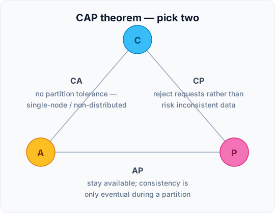
| Guarantee | Definitions |
|---|---|
| Consistency | All nodes see the same data at the same time (Wikipedia). A client perceives that a set of operations has occurred all at once (Pritchett). Any read operation that begins after a write operation completes must return that value, or the result of a later write |
| Availability | Every operation must terminate in an intended response (Pritchett). Every request received by a non-failing node in the system must result in a response |
| Partition tolerance | The system continues to operate despite arbitrary message loss (Wikipedia). Operations will complete even if individual components are unavailable (Pritchett). The cluster continues to function even if there is a "partition" — a communications break — between two nodes |
Once your network failures split your cluster, you can continue to be available and lose consistency, OR go offline and wait until failures are restored, keeping your data consistent.
BASE
| Property | Meaning |
|---|---|
| Basically available | The system does guarantee the availability of the data as regards CAP — there will be a response to any request. But that response could still be "failure" to obtain the requested data, or the data may be in an inconsistent or changing state — much like waiting for a cheque to clear |
| Soft state | Stores don't have to be write-consistent, nor do different replicas have to be mutually consistent |
| Eventual consistency | Stores exhibit consistency at some later point — e.g. lazily at read time |
Key-value stores and Redis
A key-value database, or key-value store, is a data storage paradigm designed for storing, retrieving and managing associative arrays — a data structure more commonly known today as a dictionary or hash. Dictionaries contain a collection of objects or records, which in turn have many different fields within them, each containing data. These records are stored and retrieved using a key that uniquely identifies the record and is used to quickly find the data.
Any request for the data without the key might be a performance killer.
Redis is an open-source in-memory database project implementing a distributed, in-memory key-value store.
Persistence is achieved in two different ways:
- Snapshotting — a semi-persistent durability mode where the dataset is asynchronously transferred from memory to disk from time to time, written in RDB dump format
- AOF — since version 1.1, the safer alternative: an append-only file (a journal) that is written as operations occur
Redis supports different kinds of data structures — strings, lists, maps, sets, sorted sets, hyperloglogs and more. Redis maps keys to types of values, and an important difference between Redis and other structured storage systems is that Redis supports not only strings, but also abstract data types — including sets of strings (collections of non-repeating unsorted elements).
Document-oriented databases
Document databases are inherently a subclass of the key-value store — but the difference is the one that matters for design:
In a key-value store the data is considered inherently opaque to the database, whereas a document-oriented system relies on internal structure in the document in order to extract metadata that the database engine uses for further optimization.
Contrast with the relational model. Relational databases generally store data in separate tables defined by the programmer, and a single object may be spread across several tables. Document databases store all information for a given object in a single instance, and every stored object can be different from every other. This eliminates the need for object-relational mapping while loading data into the database.
Addressing. Documents are addressed via a unique key representing that document — a simple identifier, typically a string, a URI, or a path. The database typically retains an index on the key to speed up retrieval, and in some cases the key is required to create or insert the document.
Querying — where document stores really diverge from key-value stores. Beyond simple key-to-document lookup, a document database offers an API or query language that lets you retrieve documents based on content or metadata — for example, all documents with a certain field set to a certain value. The set of query features available, and the expected performance of those queries, varies significantly from one implementation to another, as do the indexing options.
The concrete illustration of why the metadata matters:
In theory the values in a key-value store are opaque black boxes. They may offer search systems similar to a document store, but with less understanding about the organization of the content. Document stores use the metadata in the document to classify the content — allowing them, for instance, to understand that one series of digits is a phone number and another is a postal code. This lets them search on those types of data: all phone numbers containing 555, which would ignore the zip code 55555.
MongoDB and BSON
One of MongoDB's key features is that it uses the BSON format — Binary JSON — a binary-encoded serialization of JSON-like documents used when storing documents in collections.
| Property | Consequence |
|---|---|
| Binary encoding of a JSON-like structure | Adds support for data types like Date and binary that aren't supported in plain JSON |
The _id field as primary key | Its value is usually a unique identifier type named ObjectId, generated either by the application driver or by the mongod service if the driver could not generate one |
| Internal indexability | BSON enables MongoDB to internally index and map document properties — and even nested documents |
MongoDB provides its own replica sets for high availability — one primary plus one or more secondaries — and, unlike the generic master-slave pattern described above, a replica set runs an automatic election to promote a new primary when the current one fails, so failover need not be manual. MongoDB scales horizontally through sharding: a chosen shard key determines how documents are range- or hash-partitioned across shards, each itself a primary with its own replicas.
It is designed to be more efficient than storing raw JSON, which is the reason for choosing a binary encoding in the first place.
Graph databases (e.g. Neo4j) round out the NoSQL taxonomy: data is modelled as nodes, edges and properties, with relationships stored and traversed directly rather than computed through joins — a real payoff for connected-data queries such as fraud rings or recommendations. They are queried with graph-native languages like Cypher, Gremlin, SPARQL or GraphQL, and a production system such as Neo4j still offers ACID transactions alongside clustering (e.g. Raft-based Causal Clustering) for high availability.
9.7 Search
Coverage note. The Search deck is almost entirely diagrams — 47 pages yielded ~340 words. The extractable substance concerns analysis at index time, which is the conceptual core anyway:
- Stemming — "foxes" can be stemmed, reduced to its root form, to become "fox". Similarly "dogs" could be stemmed to "dog"
- Synonyms — "jumped" and "leap" are synonyms and can be indexed as just the single term "jump"
Beyond stemming and synonym folding, ranking itself rests on three named models worth knowing: the Boolean model, which ranks purely on the presence or absence of query terms in a document; the Vector Space Model, which represents both documents and the query as vectors in a shared term space and ranks by the cosine similarity (the angle) between them; and TF-IDF (term frequency × inverse document frequency), which weights a term higher the more often it appears in a document but lower the more documents across the corpus contain it — the classic building block underneath most relevance scoring.
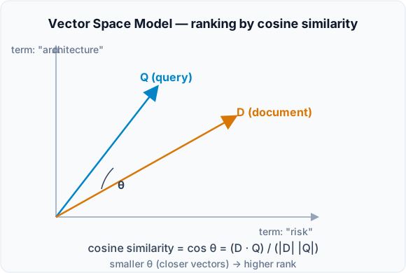
Exercises — Module 9
Task. Size and cost a cloud deployment for Lumen Diagnostics. Output: deployment view (AWS, Azure or GCP stencils), availability estimate with the series/redundancy/SLA rules below, monthly and yearly run cost.
- Read the Lumen Diagnostics case
- Draw a deployment view in AWS, Azure or GCP
- Any notation is fine; use that cloud's stencils
- draw.io, Lucidchart, Microsoft icons in Visio, or cloudcraft.co (AWS)
- Estimate availability (this is the slow part if done properly)
- Series (single points of failure):
A1 × A2 × ... × An - Redundancy: m identical copies give
1 - (1 - A1)^m - Per component: infrastructure × software (
Ai × As) - Use published cloud SLAs; read the exclusions (each cloud defines "unavailability" differently)
- EC2: 99.99% is region-based, only with 2+ AZs, and does not rise at 3+ AZs. More nines means more regions.
- Series (single points of failure):
- Monthly and yearly running cost