What you'll be able to do
- Test whether a workload needs big-data technology at all, from its volume, velocity and variety, and name the modern stack — object storage, open table formats, warehouses and lakehouses, change data capture — if it does
- Choose file formats and compression for raw and analytical data from the access pattern
- Choose a messaging model — queue, publish-subscribe or log — and a broker, and apply the polling consumer, transactional outbox and idempotent receiver patterns to an integration
- Explain CAP, PACELC and BASE, and decide per operation where a system may serve stale data and where it must refuse
- Choose between relational, key-value, document, wide-column and graph stores, and a replication topology, from the data's shape and consistency needs
- Decide whether a feature needs vector or hybrid search, choose where the vectors live, and evaluate retrieval with recall@k and nDCG
- Record data and integration choices as ADR-style decisions traced to ASRs
Part 1 decided where Lumen runs and what it costs to run. This part decides how its data is stored, moved and searched: the transactional store behind every booking, the search index behind F01, the reporting store behind the financial and partner reports, and the integrations that bring referrals in and send notifications out. Most of the technologies below were built for problems far larger than Lumen's, and you need to know them for exactly that reason — so you can say why a design does not need them, with numbers, and pick the one piece of each family that it does. The short Task at the end asks for those choices as decision records.
Data and analytics
Big data characteristics
| V | Meaning |
|---|---|
| Volume | With every year, the meaning of what big data is changes |
| Variety | Digitally sourced data has variety in that it is collected with varying degrees of structure. Data can be heavily unstructured — audio, video and social media posts. A company can gather more structured data on customers' clicks on its website, or a person can track heart rate and physical activity with a wearable — but data must then be organized in order to be useful. Multi-structured data can involve combinations of structured and unstructured data, organized by similar attributes |
| Velocity | Increasingly, businesses have stringent requirements from the time data is generated to the time actionable insights are delivered to users. Therefore data needs to be collected, stored, processed and analyzed within relatively short windows — ranging from daily to real-time |
Major cloud providers enable processing of huge volumes of data on demand, and every year data processing frameworks are updated and capabilities added.
Using an RDBMS for huge volumes is not recommended — but where "huge" begins keeps moving. A modern relational database with table partitioning routinely holds billions of rows, so check the actual volume and growth before assuming you need big-data tooling at all.
Data forms
In order to work efficiently with data we have to understand data content.
| Form | Characteristics |
|---|---|
| Structured | Highly organized information that uploads neatly into a relational database — think traditional row database structures — lives in fixed fields, and is easily detectable via search operations or algorithms. Relatively simple to enter, store, query and analyze, but it must be strictly defined in terms of field name and type (alpha, numeric, date, currency), and as a result is often restricted by character numbers or specific terminology. Analysts typically use SQL |
| Unstructured | May have its own internal structure but does not conform neatly into a spreadsheet or database. While unruly in nature it is also incredibly valuable and increasingly available in the form of complex sources: web logs, images, video, email, customer service interactions, sales automation, social media. Most business interactions, in fact, are unstructured in nature. The fundamental challenge is that these sources are difficult for non-technical business users and data analysts alike to unbox, understand and prepare for analytic use. Beyond structure there is the sheer volume — because of this, current data mining techniques often leave out valuable information and make analyzing unstructured data laborious and expensive |
| Semi-structured | Maintains internal tags and markings that identify separate data elements, which enables information grouping and hierarchies. Both documents and databases can be semi-structured — JSON and XML are the everyday examples. It is a smaller share of most organisations' data than the other two forms, but has critical business usage cases |
File formats
Multiple storage formats are suitable for HDFS and for the cloud object storage that has largely replaced it — plain text, rich formats like Avro and Parquet, Hadoop-specific formats like sequence files — each with pros and cons depending on use case. Classify them into two simple categories: raw data formats and processed data formats.
The access patterns differ, and so the formats should differ. For processing raw data we usually use all the fields, so the underlying storage must support that efficiently. But we access only a few columns of processed data in analytical queries, so the storage should handle that in the most efficient way in terms of disk I/O.
Raw data formats
| Format | Notes |
|---|---|
| Plain text file | A very common data-lake use case is storing log files or other plain text files with unstructured data. These text files could easily eat up whole disk space, so proper compression is required depending on use case |
| Structured text data | More sophisticated text files having data in a standardized form — CSV, TSV, XML or JSON |
| Binary files | Images, videos stored as-is |
| Avro | Language-neutral data serialization. Avro-formatted data can be described through a language-independent schema, so it can be shared across applications using different languages. Avro stores the schema in the header of the file, so data is self-describing. Avro files are splittable and compressible, making it a good candidate for distributed storage. Schema evolution — the schema used to read an Avro file need not be the same as the schema used to write it, making it possible to add new fields. The schema is usually written in JSON, and can be generated from Java POJOs using Avro-provided utilities |
Processed data formats
| Format | Notes |
|---|---|
| Columnar formats (general) | They eliminate I/O for columns that are not part of the query, so they work well for queries requiring only a subset of columns. They provide better compression because similar data is grouped together |
| Parquet | A columnar format. Well suited for data warehouse kind of solutions where aggregations are required on certain columns over a huge set of data. Provides very good compression, especially with codecs such as Snappy or zstd — how much depends on the data, so measure it on a sample. Can be read and written using the Avro API and Avro Schema. Also provides predicate pushdown, further reducing disk I/O cost |
| ORC | Optimized Row Columnar — the other widely used columnar format, from the Hive ecosystem, with similar compression and predicate pushdown plus lightweight built-in indexes |
Columnar vs row formats — Parquet vs Avro. Columnar formats are generally used where you need to query only a few columns rather than all the fields in a row, because their column-oriented storage pattern suits that. Row formats are used where you need to access all the fields of a row. So generally Avro is used to store the raw data, because during processing usually all the fields are required.
Compression. Big data solutions should process large amounts of data in quick time. Compressing data speeds up I/O operations and saves storage space — but this could increase processing time and CPU utilization because of decompression. So balance is required: more compression means smaller data size but more processing and CPU utilization.
Compressed files should also be splittable to support parallel processing. If a file is not splittable it means we cannot input it to multiple tasks running in parallel — and hence we lose the biggest advantage of parallel processing frameworks.
Which codecs qualify: a gzip-compressed file is not splittable and must be read by a single task; bzip2 is splittable but slow; Snappy, LZ4 and zstd are not splittable as whole compressed files, but are splittable when used inside a container format that compresses block by block — Parquet, ORC, Avro or SequenceFile. In practice: pick the container format first, then the fastest codec it supports.
From data to insight
| Level | Definition |
|---|---|
| Data | The representation of facts as text, numbers, graphics, images, sound or video. Technically data is the plural of the Latin datum, "something given", though people commonly use the term as singular. Facts are captured, stored and expressed as data. Data is the raw material we interpret as data consumers to continually create information. Data is not automatically right: capture, entry and measurement errors are common, which is why the next level begins by cleaning it |
| Information | Data that has been "cleaned" of errors and further processed in a way that makes it easier to measure, visualize and analyze for a specific purpose. Depending on that purpose, processing can involve different operations — combining different sets of data (aggregation), ensuring the collected data is relevant and accurate (validation). For example, we can organize data in a way that exposes relationships between seemingly disparate and disconnected data points. By asking relevant questions about who, what, when and where, we derive valuable information. Information can be wrong |
| Knowledge | Information becomes knowledge when we get to the question of how. When we don't just view information as a description of collected facts but also understand how to apply it to achieve our goals, we turn it into knowledge. This knowledge is often the edge that enterprises have over their competitors |
| Insight | The top of the pyramid — Ackoff's DIKW (1989) names this level wisdom: the judgement to decide what to do, and why. In analytics this is where insight lives — as we uncover relationships that are not explicitly stated as information, we get deeper insights. Applying data science allows us to derive historical, predictive or prescriptive insights, answering "Why did it happen?", "What is likely to happen?", "What should we do to make things happen?" |
While traditional analytics allows us to look backward and discover patterns that happened in the past, modern predictive analytics and machine learning techniques allow us to create a forward-looking ("windshield") view.
Analytics maturity
| Stage | Question | Techniques and characteristics |
|---|---|---|
| Descriptive | What happened | Analyze and summarize historical data; observed customer behaviour; non-traditional data sources such as web crawling and social listening |
| Diagnostic | Why did it happen | Identify the cause of trends and outcomes; observed customer behaviour; the same non-traditional sources |
| Predictive | What could or will happen | Predict outcomes based on the past; forward-looking view of current and future customer view; sentiment scoring; graph analysis and NLP to identify hidden relationships; dual-objective models; behavioural economics |
| Prescriptive | What should we do | Recommend right or optimal actions or decisions; real-time product and service propositions; rapid evaluation of multiple what-if scenarios; optimization of decisions or actions |
| Cognitive | How can we adapt to change | Monitor, decide and act autonomously or semi-autonomously; monitor results on a continuous basis; dynamically adapt based on changing environment and improved predictions; agent-based and dynamic simulation models |
Big data solution requirements
Scalability. The solution must be scalable — but how scalable, and to which capacity? This question can be answered by dividing data and applications into categories, creating a predictive model of capacity needs for each category based on expected growth, and aggregating the results.
Scalability is not just about the size of storage; it has wider implications. The throughput and the speed of access must be scalable. In addition, the system should be able to scale operationally — that is, to grow quite large without a huge increase in dedicated staff.
Self healing. A well-designed big data solution must accommodate component failures and heal itself without human intervention.
The Hadoop stack, and what replaced it
For about a decade from 2006, "big data" meant Apache Hadoop. Its parts still name the problems every data platform solves.
| Component | What it is | Why it mattered |
|---|---|---|
| HDFS | A distributed file system: large files split into big blocks, each block copied to (by default) three commodity machines, with a NameNode holding the metadata | Made petabytes cheap to keep on ordinary servers, and survived disk and node failure as a routine event |
| MapReduce | A programming model: map turns input records into key-value pairs, the framework shuffles and sorts them by key, and reduce aggregates each key's values. The framework sends the work to the nodes that hold the data | Let ordinary programmers run fault-tolerant batch jobs across thousands of machines — "move the computation to the data" |
| YARN | The cluster resource manager from Hadoop 2 onward, scheduling containers for MapReduce and other engines | Separated resource management from the processing model, so other engines could share the cluster |
| Hive | SQL (HiveQL) over files in HDFS, compiled into distributed jobs, with a metastore recording tables, columns and partitions | Opened the data to analysts who knew SQL. Its metastore and partitioned directory layout became the template for later table formats |
| Spark | A general execution engine that plans a whole job as one graph of stages and keeps intermediate results in memory where it can, instead of writing them to disk between every step as MapReduce does | Much faster for multi-step and iterative work, with one engine for SQL, streaming and machine learning. It replaced MapReduce, not the whole platform |
Three lessons outlived the stack: keep computation close to the data; treat node failure as normal; and lay files out — columnar formats, partitions on the columns you filter by — for the queries you will actually run.
What changed is where the pieces run. The modern stack separates storage from compute:
- Object storage (Amazon S3, Azure Data Lake Storage, Google Cloud Storage) replaced HDFS: cheaper, effectively unlimited, and durable without running a cluster
- Open table formats — Apache Iceberg, Delta Lake, Apache Hudi — add what a folder of Parquet files lacks — atomic commits, schema and partition evolution, time travel — through table-level metadata (snapshots or a transaction log), so several engines can share one copy safely. They replaced Hive's directory-based partition tracking; a catalog (Hive Metastore, AWS Glue, Unity Catalog or an Iceberg REST catalog) still names the tables
- Cloud data warehouses (BigQuery, Snowflake, Amazon Redshift, Microsoft Fabric) and lakehouses (Databricks, or a warehouse querying Iceberg tables in object storage) replaced Hive on Hadoop for SQL analytics: compute that starts in seconds, scales per query and bills by use
- Change data capture (CDC) — reading the transactional database's own change log, with a tool such as Debezium or a managed service such as AWS Database Migration Service, and applying every insert, update and delete to the analytical store — is replacing the nightly bulk extract wherever freshness matters. Reports trail the operational system by minutes, and analytical queries never touch the production database
The modern analytical path: no cluster to run, one copy of the data, and the transactional database is read only through its change log.
Does Lumen need this? Run the numbers before the technology. Lumen performs ~350,000 studies a month and keeps 6.5M live records: 6.5M records × ~4 KB with indexes ≈ 26 GB, plus ≈ 19 GB of stage history (2.1M changes a month × 18 months × ~0.5 KB, assumed) — roughly 45 GB. Its heaviest write stream is the 2.1M notifying stage changes a month: 84,000 per operating day (2.1M ÷ 25), and about 10,000 in the busiest hour if they peak like referrals at 12% — under three writes a second. Volume, velocity and variety are all small: the records are structured, and the case puts no images in scope; they stay in the centres' imaging archives. One managed relational database, with a standby for availability and a read replica, carries the load with room to spare, and a separate reporting store — columnar files queried by a serverless engine, or a small warehouse, fed by CDC or a nightly extract — keeps analytical queries off it. There is no big-data platform in Lumen's architecture; proposing one would add cost to a bid scored 25% on five-year cost. Revisit only if a requirement changes the numbers — years of history analysed at once, or analytics on clinical content.
Message-oriented middleware
Using a MOM system, a client makes an API call to send a message to a destination managed by the provider. The call invokes provider services to route and deliver the message.
Channels, also known as queues, are logical pathways that connect the programs and convey messages. In Hohpe and Woolf's description in Enterprise Integration Patterns, a channel behaves like a collection or array of messages — but one that is "magically shared across multiple computers and can be used concurrently by multiple applications."
Message Brokers are a subset of MOM. Brokerless solutions are another subset. Messaging tends to concentrate on the reliable exchange of messages around a network, using queues as a reliable load balancer and topics to implement publish and subscribe.
An ESB can be used as MOM, however it provides a lot of other services that are out of MOM scope. An ESB typically adds features beyond messaging such as orchestration, routing, transformation and mediation.
Three common misconceptions about queues, and their corrections:
- "A queue is a load balancer." It's better to use load balancers for balancing the load, not a message queue. That said, if messages are arriving at a queue faster than the consumer can process them, we can start multiple instances of the consumer process and the message broker will "balance the load" by distributing the messages among the available consumers
- "A queue is a single point of failure." A message queue, as an architecture element, can be configured for high reliability and availability — clustering, replicated queues, guaranteed delivery
- "A queue in the path makes the system slow." With several consumers working in parallel, a correctly designed event-driven architecture can be performant
Standards
AMQP
AMQP stands for Advanced Message Queuing Protocol.
- A binary, application-layer protocol (wire-level)
- Does not have a standard API
- Open standard: ISO/IEC 19464 — which standardises AMQP 1.0 (an OASIS standard since 2012, ISO/IEC since 2014)
- A lot of brokers implement it and there are a lot of native clients
History: AMQP was originated in 2003 by John O'Hara at JPMorgan Chase in London. In 2005 JPMorgan Chase approached other firms to form a working group, which grew to 23 companies over the next years. Previous versions were 0-8 (June 2006), 0-9 (December 2006), 0-10 (February 2008) and 0-9-1 (November 2008) — and these earlier releases are significantly different from the 1.0 specification.
The difference matters in practice, because "AMQP" usually means one of two different protocols. AMQP 0-9-1 defines a broker model — exchanges that route messages into queues according to bindings — and is RabbitMQ's native protocol. AMQP 1.0, the ISO standard, is a symmetric message-transfer protocol between peers and defines no exchanges or bindings; how a broker routes messages is left to the broker. RabbitMQ 4.x supports both, as do several other brokers. Everything below about exchange types is AMQP 0-9-1.
Exchange types (AMQP 0-9-1)
| Exchange | Routing behaviour |
|---|---|
| Direct | Messages are routed to the queues whose binding key exactly matches the routing key of the message. The default exchange is a pre-declared direct exchange with no name, usually referred to by the empty string "". When you use the default exchange, your message is delivered to the queue with a name equal to the routing key of the message — because every queue is automatically bound to the default exchange with a routing key the same as the queue name |
| Fanout | Routes messages to all of the queues bound to it. Using it we can implement the publish-subscribe pattern, where each consumer listens to its own queue. The fanout copies and routes a received message to all bound queues regardless of routing keys or pattern matching — keys provided will simply be ignored |
| Topic | Does a wildcard match between the routing key and the routing pattern specified in the binding |
| Headers | Ignores the routing key and routes on message header values matched against the binding's arguments — all of them or any one of them |
JMS
Java Message Service (JMS) API. Versions: 1.0.2B (June 26, 2001), 1.1 (April 12, 2002), 2.0 (May 21, 2013). After Java EE moved to the Eclipse Foundation, JMS continued as Jakarta Messaging: version 3.0 (2020) renamed the package from javax.jms to jakarta.jms, and 3.1 (2022) followed with Jakarta EE 10. New Java code targets Jakarta Messaging.
- The JMS specification was originally developed to allow Java applications access to existing MOM systems. Since its introduction it has been adopted by many existing MOM vendors, and has been implemented as an asynchronous messaging system in its own right
- In JMS, APIs are specified, but the message format is not. Unlike AMQP, JMS has no requirement for how messages are formed and transmitted. Essentially, every JMS broker can implement the messages in a different format. They just have to use the same API
- The single biggest change in JMS 2.0 is a new API for sending and receiving messages that reduces the amount of code a developer must write
JMS elements
| Element | Definition |
|---|---|
| JMS provider/broker | An implementation of the JMS interface for message-oriented middleware. Providers are implemented as either a Java JMS implementation or an adapter to a non-Java MOM |
| JMS client | An application or process that produces and/or receives messages |
| JMS producer/publisher | A JMS client that creates and sends messages |
| JMS consumer/subscriber | A JMS client that receives messages |
| JMS message | An object that contains the data being transferred between JMS clients |
| Destinations | JMS queue or topic |
Others
Two more protocols are worth knowing. STOMP is a simple wire-level, text-oriented messaging protocol — easy to implement and debug, but far less structured than AMQP's binary framing. MQTT (formerly MQ Telemetry Transport) is a lightweight publish/subscribe protocol built on top of TCP/IP that is more efficient than HTTP-based alternatives; it has become the de facto standard for constrained and embedded IoT devices, offering basic authentication and, where link security is needed, SSL/TLS encryption at the cost of added overhead.
Message brokers
A message broker is an intermediary that sits between senders and receivers: it accepts, stores and routes messages, and can translate between the messaging protocols each side speaks. Most brokers add further services on top — persistence, acknowledgement and redelivery, routing rules and access control.
Persistence. A message can be published either with a delivery mode set to persistent or transient.
How brokers treat the two differs by product and version, so check yours; the classic RabbitMQ behaviour illustrates the idea. A persistent message is written to disk as soon as it reaches the queue, so it survives a broker restart. A transient message may also reach disk, but only when the broker pages it out to relieve memory pressure — it does not survive a restart. Writing a message to disk does not remove it from memory: the broker keeps a cache of messages in RAM for fast delivery, and "paging out" means moving messages from that cache to disk. Newer queue types narrow the distinction — RabbitMQ's replicated quorum queues, for example, store every message durably.
Implementations — open-source, proprietary and cloud-oriented; the list is not exhaustive: RabbitMQ, Apache ActiveMQ (Classic and Artemis, the successor to HornetQ), Apache Kafka, Apache Pulsar, Apache Qpid, NATS, IBM MQ (formerly WebSphere MQ), Oracle Advanced Queuing, Microsoft Message Queuing (Windows legacy), and cloud services such as Amazon SQS, Amazon MQ, Azure Service Bus, Azure Event Hubs and Google Cloud Pub/Sub. Task-queue frameworks such as Celery are not brokers themselves — they run on top of one.
In addition, hardware-based messaging middleware exists: Solace, for example, offers messaging appliances alongside its software and cloud brokers.
RabbitMQ
- Open source
- Written in Erlang and built on the OTP (Open Telecom Platform)
- Developed by Pivotal from 2013, then VMware; part of Broadcom since its 2023 acquisition of VMware
- Extensible plug-in architecture
- Multiple protocols — AMQP 0-9-1 and AMQP 1.0 natively in 4.x, plus MQTT and STOMP
Clustering and replication. Typically you would use clustering for high availability and increased throughput, with machines in a single location.
A classic queue within a RabbitMQ cluster lives on a single node — the node on which it was declared — whereas exchanges and bindings exist on all nodes. A classic queue is therefore lost to its consumers if that node fails.
For availability, queues are replicated across nodes. Older RabbitMQ versions did this by mirroring classic queues; that feature was deprecated and then removed in RabbitMQ 4.0 (2024). Its replacements are:
- Quorum queues — replicated queues based on the Raft consensus algorithm. Each has one leader and several followers; a message is confirmed once a majority of replicas hold it, and if the leader fails a follower is elected in its place. Use an odd number of replicas, typically three or five
- Streams — a replicated, append-only log with non-destructive reads, closer to Kafka's model, for fan-out and replay
Replication enhances availability but does not distribute a single queue's load across nodes — the leader still handles all of that queue's traffic, and every replica stores every message. To spread load, spread queues across nodes.
Apache Kafka
Kafka is built around a log, an idea borrowed from databases. A database records every change in its transaction log (also called its journal or binary log) so that, after a crash or a hardware failure, it can replay or undo work and keep its ACID guarantees. On disk that log is simply an append-only file of changes.
Topics and partitions (after the Apache Kafka documentation). Producers publish messages to a named topic, and Kafka stores each topic as a partitioned log: every partition is an ordered, append-only sequence of messages that is never modified once written.
Any number of consumers — none, one or many — can subscribe to the same topic.
Reading a message does not delete it. Kafka keeps every message for a configured retention period, whether or not anyone has consumed it.
What Kafka tracks per consumer is essentially one number per partition: the consumer's position in the log, its "offset" — and the consumer controls it. Normally a consumer advances its offset as it reads, but it can also move it: reset to an older offset to reprocess history, or skip ahead.
Each consumer group reads every partition of the topic; within a group, each partition is assigned to one consumer at a time.
Partitioning does two jobs. It lets a topic outgrow a single server — one partition must fit on the brokers that host it, but a topic can have as many partitions as its volume needs — and it makes the partition the unit of parallelism.
Each partition is copied to a configurable number of brokers. One copy is the leader: writes, and by default reads, go to it. The others are followers that replicate the leader, and if the leader fails, a follower takes over automatically. (Since Kafka 2.4, consumers can also be configured to read from a nearby follower, to save cross-zone traffic.)
Cluster metadata — which broker leads which partition — used to live in Apache ZooKeeper. Kafka now manages it itself through KRaft, a built-in Raft-based controller quorum, and Kafka 4.0 (2025) removed ZooKeeper support entirely; ZooKeeper-based clusters must migrate to KRaft before upgrading.
Consumer groups. One abstraction, the consumer group, covers both queueing and publish-subscribe.
Every consumer joins a named group, and each message on a topic reaches exactly one consumer in every group that subscribes to it. A group's consumers can be spread across processes and machines.
- Put all the consumers in one group and the messages are shared out among them — a queue
- Give each consumer its own group and every consumer receives every message — publish-subscribe
Because each partition is assigned to one consumer within a group, a group's parallelism is capped by the topic's partition count — a tenth consumer on a nine-partition topic sits idle. Choose partition counts with future consumer scale in mind. A second option, share groups ("queues for Kafka"), became production-ready in Kafka 4.2 (2026): consumers acquire and acknowledge individual records rather than owning partitions, so more consumers than partitions can work one topic — at the cost of per-partition ordering.
ZeroMQ
ZeroMQ is designed to be faster, but it lacks many of the broker functions the others provide — there is no broker to lose, and no broker to rely on. Published throughput figures vary sharply with message size, so benchmark at your own payload size rather than trusting a headline number.
AWS messaging
Fully managed messaging services: Amazon SQS, Amazon SNS, Amazon EventBridge (an event bus with rule-based routing), Amazon Kinesis, Amazon MSK (managed Kafka), Amazon MQ (managed ActiveMQ and RabbitMQ) and AWS IoT Core's message broker. For messages to people rather than services — the email and SMS notifications most business systems need — use Amazon SES for email and AWS End User Messaging for SMS. Amazon Pinpoint, the engagement platform that once bundled these channels, reached end of support on 30 October 2026; its SMS, voice and push APIs continue under AWS End User Messaging.
SQS — Simple Queue Service
Amazon SQS is a fully managed message queuing service that enables you to decouple and scale microservices, distributed systems, and serverless applications.
| Queue type | Characteristics |
|---|---|
| Standard queue | Higher throughput, at-least-once delivery, best-effort ordering |
| FIFO queue | Ordering preserved, exactly-once processing, limited throughput |
Visibility timeout — how to set it. SQS does not delete a message when a consumer receives it; it hides it for the visibility timeout (30 seconds by default, up to 12 hours). If the consumer deletes the message within that window, processing is done; if not, the message reappears for another consumer — which is how SQS recovers from a crashed consumer. Messages are processed at different speeds, and getting this wrong hurts in both directions.
Consider the typical scenario of processing files: we store the file to S3 and send its reference to a queue. Usually the file size is up to 100 KB — however, it's even possible to get a file up to 1 GB (a huge attachment), and processing it could take a while. With a small visibility timeout it could cascade: the large file reappears before its first consumer finishes, a second consumer starts on it too, and so on, choking up all the threads. With a large visibility timeout it could be a very delayed failover: when a consumer dies mid-task — routine when autoscaling removes instances — its message stays hidden until the long timeout expires.
The remedy is not a single magic number: set a timeout that fits the typical message, have consumers extend the visibility of a long-running message while they work on it (a heartbeat calling ChangeMessageVisibility), make consumers idempotent, because standard queues deliver at least once, and cap retries with a dead-letter queue.
Dead-letter queues capture messages that cannot be processed successfully after a set number of receives. Lambda integrates with SQS as an event source.
Virtual queues are a feature of the AWS Temporary Queue Client library for Java rather than of SQS itself: the client multiplexes many short-lived logical queues over one real queue. They build on the Return Address enterprise integration pattern — worth knowing when you need request/reply semantics over a queue without provisioning a queue per requester.
SNS — Simple Notification Service
A highly available, durable, secure, fully managed pub/sub messaging service that enables you to decouple microservices, distributed systems and serverless applications.
The architecturally interesting feature is filter policies: a subscription carries a filter expressed as JSON, and SNS matches it against the message attributes — or, since 2022, the message body — of each published message, delivering only what matches. That moves routing logic out of consumers and into the messaging layer — the same concern AMQP 0-9-1 solves with topic and headers exchanges.
Kinesis
Amazon Kinesis makes it easy to collect, process and analyze real-time streaming data so you can get timely insights.
Two properties worth carrying into a design:
- Kinesis + Lambda have a "native" integration — you get stream processing without having to write polling code
- Amazon Data Firehose (called Kinesis Data Firehose until 2024) is for loading data from a Kinesis data stream into data stores and analytics tools — the managed sink, as opposed to the stream itself
Kinesis Data Streams gained higher fan-out and faster stream reads through enhanced fan-out, which removes the shared-throughput constraint when several consumers read the same shard.
Integration patterns for an extract-only source
Brokers move messages; three patterns decide whether an integration built on them is correct. All three are needed the moment a source cannot push events — and Lumen's referral system publishes a change extract every 15 minutes, with no event or webhook interface.
- Polling consumer (Hohpe & Woolf, Enterprise Integration Patterns). The consumer fetches on its own schedule: here, each new extract, in order, recording the last one applied as a high-water mark so that a restart resumes rather than repeats. The 15-minute extract interval sets a latency floor: a change made just after an extract is cut waits up to 15 minutes for the next one, plus processing — about 20 minutes worst case. That is why Module 3's QA11 is measured from the extract, not from the change; if Lumen needs "within 15 minutes of the change", ask for an event feed or a shorter interval, and raise it as a clarification rather than hide it in the design
- Idempotent receiver (Hohpe & Woolf; also called an idempotent consumer). Applying the same change twice must leave the same state as applying it once. Extracts overlap, retries replay them and queues deliver at least once, so key every change by the referral's identifier and a version or timestamp from the source, and skip any change that is not newer than what is stored. Duplicates become no-ops instead of double bookings or repeated SMS
- Transactional outbox (Richardson, Microservices Patterns). When a state change must also emit a message — a stage change that notifies the patient — write the change and an outbox row in the same database transaction; a relay then publishes outbox rows to the queue and marks them sent. Without it, a crash between commit and publish loses the notification, and publishing before a commit that later rolls back notifies a change that never happened. The relay may publish a row twice, so the consumer must be idempotent too
Every step that can repeat is idempotent, and every message that must not be lost leaves the database in the same transaction as the change that caused it.
Conflicts are a business rule, not a technical one: the case asks for amendments to be "merged according to a defined policy", with alerts. Write the policy down field by field — for example, the referral system wins on clinical details and the platform wins on the booking — and alert the referral desk whenever an incoming change touches a confirmed booking.
NoSQL
Why relational databases won — and why NoSQL appeared
Even though SQL databases appeared after hierarchical and network databases, they won the battle and dominated for decades as mainstream data storage. Why?
- First, the relational data model is built on a strong mathematical foundation — normalization theory
- It provides ACID guarantees on data updating and reading, which allows you to rely on data consistency
- It provides vertical scaling, which worked — and still works to some extent — well in many cases
However, not so many years ago a whole family of NoSQL databases appeared. They might be considered successors of the hierarchical and networking databases designed in the 1960s. Why?
- Because the world changed. Nowadays we have significantly increased amounts of data that can barely be handled by a single server. In addition, we want this data to be handled immediately — 20 years ago the creation of a complex report might take several hours and that was OK; now we want results immediately
- The business wants 100% availability, which can't be reached with a single server: downtimes are needed to maintain hardware, install updates, change database schemas
- In many cases we must deal with poor connections between servers and restrictions of network protocols
So we need horizontal scaling and clustering to handle these requirements. But traditional SQL databases were not designed to work in a cluster — and the root cause is the ACID guarantees, which are expensive to coordinate across nodes.
That root cause is a cost, not an impossibility. Distributed SQL databases — Google Spanner, CockroachDB, YugabyteDB, Amazon Aurora DSQL — provide ACID transactions across a horizontally scaled cluster, paying for it in cross-node coordination latency. And a single well-sized relational server, with read replicas, still covers most business systems.
Scalability techniques
Two important techniques for horizontal scalability
| Technique | Detail |
|---|---|
| Partitioning (sharding) | The database can be partitioned over servers using a partitioning key that is available in nearly every transaction — to avoid sending the transaction to every server. Partitioning allows the database transaction load to be split over multiple servers, increasing the throughput of the system |
| Replication | Each partition can be replicated across at least two physical servers. Replication is useful for failure recovery, and can also provide scalability for frequently-read data because the load can be split over the replicas. But unlike partitioning, replication increases the cost of writes, so it should only be used as appropriate. And if you wait for replication to another server before transaction commit, the servers must be close — on the same LAN or, in the cloud, in different availability zones of one region, where synchronous replication is routine. Replication to a distant region for disaster recovery is usually asynchronous, so that every commit does not wait on a long round trip; the price is that the last few transactions can be lost in a regional failover (some globally distributed databases accept the latency instead, to stay consistent) |
Two important techniques for vertical scalability
| Technique | Detail |
|---|---|
| RAM instead of disk | RAM should be used to store the database. Disk should only be used for backups and possibly for logging — as Jim Gray put it in 2006, "disk is tape". If the database is too big to fit in the collective RAM and SSD of all the database servers you can afford, then a conventional distributed DBMS may be a better choice |
| Minimal durability overhead | There must be minimal overhead for database durability. Durability can be guaranteed by logging to disk and doing online backups in the background. You might even let the system log to disk after the transaction completes, depending on your comfort level. Alternatively, for many applications you can achieve acceptable durability by completing the replication to another server before returning from the transaction. For clinical or financial records — Lumen's confirmed appointments, for example — acknowledging a write before it is durable means a crash can silently lose confirmed bookings: fix the acceptable data loss (the RPO) first, and relax durability only within it |
When these vertical scaling techniques are used, the database system becomes CPU-limited instead of disk-limited.
Sharding approaches:
- Split data by attributes between different nodes — might help, however it is not scalable enough in many cases
- Split data by some attribute's value — good for dynamic scaling, however we should know on which server our data is
Primary-replica replication
Historically called master-slave replication; current database documentation uses primary and replica.
Benefits
- Analytic applications can read from the replica(s) without impacting the primary
- Backups of the entire database with relatively no impact on the primary
- Replicas can be taken offline and synced back to the primary without any downtime
- Replicas can be smaller and cheaper than the primary, and can be added or removed as read load changes
Every write funnels through one primary; reads can fan out to any replica — which is exactly why a primary failure is the single point of failure this topology has to plan around.
Drawbacks
- In the instance of a failure, a replica has to be promoted to primary to take over its place. Unless failover is automated — as managed database services (e.g. Amazon RDS Multi-AZ) and tools such as Patroni do — that promotion is a manual step
- Downtime and possibly loss of data when a primary fails, depending on whether replication was synchronous
- All writes still have to be made to the primary in a primary-replica design
- Each additional replica adds some load to the primary, since the replication log has to be read and data copied
- Multi-primary is not as simple as primary-replica to configure and deploy: concurrent writes to different primaries must be coordinated or reconciled, which costs write latency, availability or conflict-resolution effort
Replication works well with sharding. A shard manager allows us to select a needed shard, and then we can select primary or replica for operations — balancing our load pretty well.
The pain point here: we must design the data structure in a way that all the information we need is stored on a single shard — otherwise we have to travel through all our shards to collect data. It will kill the performance. And note that we may have more than one primary on a shard for some systems.
Full replication across all nodes. Data is fully replicated across all nodes, with one primary copy accepting changes and multiple active replicas typically read-only. Such configurations can be a good fit for read-intensive workloads such as reporting, where readers can potentially connect to any server and execute their queries. By contrast, writers can connect only to the primary copy, causing a bottleneck in write-intensive workloads.
Relaxing ACID
To scale up write operations, or the number of nodes in a cluster beyond a certain point, you have to be able to relax the guarantees:
| Dropping | Effect | Examples |
|---|---|---|
| Atomicity | Lets you shorten the duration for which tables (sets of data) are locked | — |
| Consistency | Lets you scale up writes across cluster nodes | Riak, Cassandra |
| Durability | Lets you respond to write commands without flushing to disk | — |
| Isolation | Lets you expose every operation immediately to any other connection | — |
Wide-column databases such as Cassandra — not to be confused with the columnar file formats and analytical stores earlier in this unit, which store each column contiguously for scans — organise data into tables (historically called column families) addressed by a primary key — a partition key, which places the row on nodes, plus clustering columns, which order rows within the partition; columns are declared per table, but storage is sparse. Cassandra runs as a masterless, peer-to-peer cluster — every node is equal, nodes exchange state via a gossip protocol, and a temporarily unreachable node's missed writes are buffered as hints and replayed through hinted handoff once it rejoins. Data is distributed across nodes by consistent hashing on a token ring, and consistency is tunable per request (from ONE through QUORUM to ALL), letting the same cluster trade off availability against consistency call by call.
CAP theorem
The CAP theorem, also named Brewer's theorem after computer scientist Eric Brewer, who stated it as a conjecture in 2000, says that a distributed data store cannot simultaneously guarantee all three of the following properties. Seth Gilbert and Nancy Lynch proved it formally in 2002.
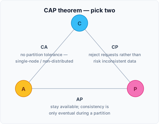
Read the triangle with care: in a distributed system partitions are not optional, so "CA" is not a real choice. The live choice is between CP and AP, and only while a partition lasts.
| Guarantee | Definitions |
|---|---|
| Consistency | All nodes see the same data at the same time. A client perceives that a set of operations has occurred all at once (Pritchett). Formally, in Gilbert and Lynch's proof: any read operation that begins after a write operation completes must return that value, or the result of a later write |
| Availability | Every operation must terminate in an intended response (Pritchett). Formally: every request received by a non-failing node in the system must result in a response |
| Partition tolerance | The system continues to operate despite arbitrary loss of messages between nodes. Operations will complete even if individual components are unavailable (Pritchett). The cluster continues to function even if there is a "partition" — a communications break — between two nodes |
Once your network failures split your cluster, you can continue to be available and lose consistency, OR go offline and wait until failures are restored, keeping your data consistent.
Brewer himself revisited the theorem in 2012 ("CAP Twelve Years Later"), warning that the "pick two of three" reading is misleading: the trade-off applies only during a partition, and is made per operation rather than once per system. Daniel Abadi's PACELC extends it to normal running: if there is a Partition, choose Availability or Consistency; Else, choose between Latency and Consistency — which is the trade-off a replicated system actually makes most of the time.
BASE
| Property | Meaning |
|---|---|
| Basically available | The system does guarantee the availability of the data as regards CAP — there will be a response to any request. But that response could still be "failure" to obtain the requested data, or the data may be in an inconsistent or changing state — much like waiting for a cheque to clear |
| Soft state | Stores don't have to be write-consistent, nor do different replicas have to be mutually consistent |
| Eventual consistency | Stores exhibit consistency at some later point — e.g. lazily at read time |
Key-value stores and Redis
A key-value store is the database form of an associative array — what most programming languages call a dictionary, map or hash. Each record, however many fields it holds internally, is stored and retrieved as a whole through one unique key, and that key is the fast path to it.
Any request for the data without the key might be a performance killer.
Redis is an in-memory key-value data store, widely used as a cache, message broker and fast database. Check its licence when you choose it: in 2024 Redis moved from an open-source licence to source-available terms, prompting the Linux Foundation fork Valkey; Redis 8 (2025) added the open-source AGPLv3 as an option. Managed cloud caches now commonly offer Valkey alongside or instead of Redis.
Persistence is achieved in two different ways:
- Snapshotting — a semi-persistent durability mode where the dataset is asynchronously transferred from memory to disk from time to time, written in RDB dump format
- AOF — since version 1.1, the safer alternative: an append-only file (a journal) that is written as operations occur
Redis supports different kinds of data structures — strings, lists, hashes, sets, sorted sets, streams, HyperLogLogs and more. What sets it apart from a plain key-value cache is that the value has a type the server understands: you can add to a set, increment a counter or pop from a list in one atomic server-side operation, instead of reading, modifying and rewriting an opaque string.
Document-oriented databases
Document databases can be seen as a special kind of key-value store — but the difference is the one that matters for design: a key-value store treats the value as opaque, whereas a document database understands the structure inside each document and uses it — to index fields, to query on them and to optimise access.
Contrast with the relational model. Relational databases generally store data in separate tables defined by the programmer, and a single object may be spread across several tables. Document databases store all information for a given object in a single instance, and every stored object can be different from every other. This eliminates the need for object-relational mapping while loading data into the database.
Addressing. Documents are addressed via a unique key representing that document — a simple identifier, typically a string, a URI, or a path. The database typically retains an index on the key to speed up retrieval, and in some cases the key is required to create or insert the document.
Querying — where document stores really diverge from key-value stores. Beyond simple key-to-document lookup, a document database offers an API or query language that lets you retrieve documents based on content or metadata — for example, all documents with a certain field set to a certain value. The set of query features available, and the expected performance of those queries, varies significantly from one implementation to another, as do the indexing options.
A concrete illustration of why that structure matters: to a key-value store, a stored record is an opaque black box, and any search over it is a search over undifferentiated text. A document database knows that one string of digits sits in a phone number field and another in a postal code field, so it can answer "phone numbers containing 555" without matching the postal code 55555.
MongoDB and BSON
One of MongoDB's key features is that it uses the BSON format — Binary JSON — a binary-encoded serialization of JSON-like documents used when storing documents in collections. It is designed to be faster to traverse and parse than raw JSON text, which is the reason for choosing a binary encoding in the first place.
| Property | Consequence |
|---|---|
| Binary encoding of a JSON-like structure | Adds support for data types like Date and binary that aren't supported in plain JSON |
The _id field as primary key | Its value is usually a unique identifier type named ObjectId, generated either by the application driver or by the mongod service if the driver could not generate one |
| Internal indexability | BSON enables MongoDB to internally index and map document properties — and even nested documents |
MongoDB provides its own replica sets for high availability — one primary plus one or more secondaries — and, unlike a primary-replica setup without automated failover, a replica set runs an automatic election to promote a new primary when the current one fails, so failover need not be manual. MongoDB scales horizontally through sharding: a chosen shard key determines how documents are range- or hash-partitioned across shards, each itself a primary with its own replicas.
Graph databases (e.g. Neo4j) round out the NoSQL taxonomy: data is modelled as nodes, edges and properties, with relationships stored and traversed directly rather than computed through joins — a real payoff for connected-data queries such as fraud rings or recommendations. They are queried with graph-native languages such as Cypher, Gremlin and SPARQL, and since 2024 with the ISO standard GQL (ISO/IEC 39075). GraphQL, despite the name, is an API query language, not a graph-database language. A production system such as Neo4j still offers ACID transactions alongside Raft-based clustering for high availability.
Search
This section covers the conceptual core of full-text search — analysis at index time, and the models used to rank results — and then vector and hybrid search, and where each earns its place. Analysis normalises text so that different forms of a word match the same entry in the index:
- Stemming — "foxes" can be stemmed, reduced to its root form, to become "fox". Similarly "dogs" could be stemmed to "dog"
- Synonyms — "jumped" and "leap" are synonyms and can be indexed as just the single term "jump"
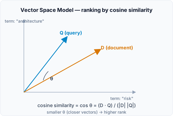
Beyond stemming and synonym folding, retrieval and ranking rest on a few named models worth knowing: the Boolean model, which only decides whether a document matches the query terms (AND, OR, NOT) and does not rank the matches at all; the Vector Space Model, which represents both documents and the query as vectors in a shared term space and ranks by the cosine similarity (the angle) between them; and TF-IDF (term frequency × inverse document frequency), which weights a term higher the more often it appears in a document but lower the more documents across the corpus contain it — the classic building block of relevance scoring. Its refinement BM25, which caps the benefit of repeating a term and normalises for document length, is the default similarity in Apache Lucene, and therefore in Elasticsearch and OpenSearch.
Lumen's F01 is mostly not text search. A referral's requirements are structured — modality, urgency, distance from the patient, date window, price — and the ranking comes from clinical match plus the Scheduling Manager's rules. What a search engine adds here is fast filtering with custom scoring, geo-distance queries, and a read model kept apart from the booking transactions; stemming and BM25 matter only for free-text fields such as practice names. Two consequences follow. The index is a copy, refreshed from the transactional store after every booking, so it is eventually consistent: a search may offer a slot taken a second ago, and the booking must re-check the slot against the database before confirming it. And at Lumen's size — under a million slot documents and about two searches a second at peak — a well-indexed relational query with a geospatial extension is a credible alternative to a separate cluster. Module 3's worked F01 assumes a dedicated search component, and part 1's worked cost model prices it at about $1,950 a month across four regions: test that assumption rather than inherit it.
Vector search: embeddings and similarity
The vector space model above represents text as sparse vectors: one dimension per vocabulary term, nearly all of them zero, weighted by TF-IDF, so two texts are similar only if they share terms. Vector search keeps the geometry and changes the vectors. An embedding model — a neural network trained on large text corpora — maps a passage to a dense vector of a few hundred to a few thousand dimensions, none of which stands for a word, placed so that passages with similar meaning lie close together. "Where do I park for my scan?" and "parking at the imaging centre" share almost no terms and score near zero under BM25; their embeddings are close.
Similarity is measured much as before:
- Cosine similarity — the cosine of the angle between two vectors, ignoring their length; the measure in the vector space model image
- Dot product — the sum of element-wise products. For vectors normalised to unit length it equals the cosine and is cheaper to compute, which is why many embedding models output unit vectors
- Euclidean distance — for unit vectors it ranks results in the same order as cosine, because squared distance = 2 − 2 × cosine
Use the measure the embedding model was trained for. Two constraints follow from how embeddings work. Vectors from different models, or from two versions of one model, are not comparable, so the query and the corpus must be embedded by the same model. And lexical precision is lost: "MRI lumbar spine" lies close to "MRI thoracic spine", which is exactly wrong when the difference matters. Hybrid search, below, exists to recover it.
Approximate nearest neighbour indexes
Finding the k nearest vectors exactly means comparing the query with every vector: flat, or brute-force, search. That is cheaper than it sounds — 20,000 vectors of 768 dimensions is about 15M multiply-adds per query, a few milliseconds on one core — and it has perfect recall, so it is the right answer for small corpora. From hundreds of thousands of vectors upwards, systems use approximate nearest neighbour (ANN) indexes, which give up a little recall for orders of magnitude in speed:
| Index | How it works | Trade-off |
|---|---|---|
| HNSW — hierarchical navigable small world graph (Malkov and Yashunin, 2016) | A layered graph in which each vector links to near neighbours; a search enters at the sparse top layer and descends greedily towards the query | Fast with high recall, and accepts inserts incrementally; the graph must sit in memory and adds overhead per vector; deleted vectors linger as tombstones until a merge, vacuum or rebuild |
| IVF — inverted file index | Clusters the vectors with k-means and searches only the few clusters nearest the query | Smaller and quicker to build than HNSW; recall depends on how many clusters are probed; clusters drift as data changes, so the index is retrained periodically |
| PQ — product quantisation (Jégou, Douze and Schmid, 2011) | Compresses each vector by splitting it into sub-vectors and replacing each with the ID of its nearest centroid | A 768-dimension float vector of 3,072 bytes can shrink to under 100 bytes, at a cost in recall; usually combined with IVF (IVF-PQ), with the top results re-ranked on full vectors |
Every index has knobs that move the same three-way trade-off between recall, latency and memory: HNSW's links per node (M) and search breadth (ef), IVF's number of probes, PQ's code size. Lower-precision vectors — 16-bit floats, 8-bit integers or single bits, with a re-ranking pass on full vectors — are common middle settings, offered in different combinations by Elasticsearch, OpenSearch and pgvector. Memory is usually the binding constraint: a million 768-dimension vectors is about 3 GB of raw floats before the graph, so at tens of millions of vectors memory, not CPU, becomes the cost line. Measure recall against flat search on your own data at your own latency target; published benchmarks use someone else's.
A vector database or an extension
| Option | Examples | Fits when |
|---|---|---|
| Extension to the relational database | pgvector for PostgreSQL, with HNSW and IVFFlat indexes, offered by the major managed PostgreSQL services | The vectors belong to rows you already store, and you want them written in the same transaction, filtered with SQL and governed like the rest of the data — backed up, access-controlled, kept in-region. Comfortable into the millions of vectors |
| Search engine k-NN | OpenSearch k-NN (Lucene and Faiss engines); Elasticsearch dense vector fields | You already run a search cluster and want lexical and vector retrieval in one query |
| Dedicated vector database | Milvus, Qdrant, Weaviate, Pinecone, and the clouds' managed vector services | Hundreds of millions of vectors, high query rates or many tenants, or features the general-purpose engines lack — at the price of another system to run, secure, back up and keep in each jurisdiction |
The rule is the one this unit applies throughout: start with the store you already run, and move only when a number requires it.
Hybrid search and rank fusion
Lexical and semantic retrieval fail differently: BM25 misses paraphrase, and embeddings blur exact terms, codes and names. Hybrid search runs both and merges the two result lists. Their scores are not comparable — BM25 scores are unbounded, cosine lies between −1 and 1 — so merging by score needs a normalisation that is fragile. Reciprocal rank fusion (RRF) (Cormack, Clarke and Büttcher, SIGIR 2009) uses ranks only:
RRF score of a document = Σ over the result lists of 1 ÷ (k + its rank in that list), with k = 60 by convention.
A help article ranked 1st by BM25 and 3rd by vectors scores 1 ÷ 61 + 1 ÷ 63 ≈ 0.0323; one ranked 2nd by vectors and absent from the BM25 list scores 1 ÷ 62 ≈ 0.0161. Agreement between the methods wins, and k damps the pull of any single top rank. Elasticsearch and OpenSearch provide RRF natively; in PostgreSQL it is a short SQL query over two ranked result sets.
Both retrievers apply the same filters, taken from the session on the server rather than from the request; fusion sees only ranks.
Filtering, tenancy and freshness
Metadata filtering. Real queries combine similarity with conditions — language, region, content type, tenant. Post-filtering retrieves the top k by similarity and then drops what fails the condition; with a selective filter it returns far fewer than k results, or none — a partner whose documents are 1% of the index gets about one result from a top-100 search. Pre-filtering applies the condition first and searches only what passes. Exact search over a small filtered set is cheap, but forcing an ANN graph to step over most of its nodes costs latency or recall, so engines now filter during the graph search: Lucene-based engines do, and pgvector added iterative index scans in version 0.8 for the same problem. Test recall with your real filters applied, not only without them.
Multi-tenancy. If partner content were ever indexed — a partner's own preparation instructions, say — QA12 applies: one partner must never retrieve another's documents. The options, from strongest isolation to weakest, are an index per tenant, a partition or namespace per tenant inside one index, and a shared index with a mandatory tenant filter. Whichever you choose, the tenant filter comes from the authenticated session on the server, never from a request parameter, and an automated test queries every tenant for another's content at each release, like QA12's existing test. Similarity is not access control: a nearest neighbour does not know who is asking.
Freshness and re-embedding. A new or changed document must be embedded and written before it can be found, so a vector index is another eventually consistent copy, refreshed like the search index above. Deletes matter as much as inserts: withdrawn preparation guidance must leave the results at once, not at the next rebuild. The expensive event is a model change. Vectors from the new model cannot be compared with the old, so every document is re-embedded and the index rebuilt — usually beside the old one, with an alias switched once the new index passes evaluation. Record the model and version on every vector. The token bill is often small — 20,000 passages of ~300 tokens is 6M tokens, under a dollar at an illustrative $0.10 per million — but at a hundred million documents re-embedding is a project, and at any size the evaluation and cut-over cost more than the tokens.
Evaluating retrieval
Measure two different things.
- Index recall: how many of the true nearest neighbours the ANN index returns, compared with flat search on the same vectors. A property of the index settings, measured automatically
- Retrieval quality: whether the results answer the query, judged by people. Build a judged set — real queries, each with the documents a domain expert marks relevant — and score every configuration (BM25, vectors, hybrid; model A against model B) on it:
- recall@k — the share of the relevant documents that appear in the top k. The metric when retrieval feeds another step: a re-ranker, a person choosing from a short list, or a language model in a RAG pipeline
- nDCG@k — normalised discounted cumulative gain (Järvelin and Kekäläinen, 2002): DCG@k = Σ relᵢ ÷ log₂(i + 1) over positions i = 1 … k, divided by the DCG of the ideal ordering, so graded relevance counts for more the higher it ranks. The metric for lists people read from the top
A few hundred judged queries are enough to tell configurations apart. Public leaderboards, such as MTEB for embedding models (Muennighoff et al., 2022), give you a shortlist, not a decision.
Where vector search helps Lumen — and where it doesn't
Helps: patient help content. The patient portal answers the same questions thousands of times a month — preparation for each modality, what to bring, parking, how to reschedule — and patients ask in their own words, not the help centre's. Hybrid search over the help articles finds "can I eat before my scan" in the fasting guidance, while the lexical half keeps modality and centre names exact. The corpus is small — say 2,000 articles in 20,000 passages (assumed) — so flat search over vectors held in pgvector, or in the search cluster's k-NN if one is kept, is enough: no ANN tuning and no new product. The same index is the retrieval half of a patient assistant that answers from the help content — retrieval-augmented generation, covered in Module 11.
Helps: mapping referral wording to codes. Referrers write "MRI L-spine ?disc", "lumbar MR" or "low back MRI with contrast"; the platform needs a modality and protocol code, and F08's clinical match depends on getting it right. Embedding the catalogue — each code's description and known synonyms, a few thousand entries (assumed) — and searching it with the referral's free text proposes the likeliest codes for the referral desk to confirm. Three design points follow. Index the catalogue, not the referrals, so no patient text is stored as vectors; embeddings can be partly inverted back to their text (Morris et al., 2023), so a stored embedding of patient data is patient data. The referral text is still patient data when it is sent to be embedded, so the embedding model runs in the region (QA05) — an embedding API in another jurisdiction is a cross-border transfer. And the result is a suggestion to a person: the desk's choices, logged, become the judged set that tracks recall@5. Whether it ever codes automatically is a clinical-safety decision, not a search one.
Doesn't help: slot availability. F01 finds slots by modality, date window, distance, urgency and price — structured fields with exact meanings. A slot is either an MRI at 10:00 within 20 km or it is not; "semantically close" means nothing, and an approximate index that misses a valid slot loses a booking. Keep F01 on the structured path — the indexed relational query, or the search index's filters and custom scoring, described above. At most, a model can turn a free-text search box into those structured fields before the query runs.
The verdict for Lumen: two optional features use vector search, at a size where flat search is enough, in stores the design already has; F01 does not use it; nothing justifies a dedicated vector database.
Check yourself
- A stakeholder asks for a Hadoop or Spark cluster "so Lumen is ready for big data". Answer with the case's numbers.
- Why is Parquet a better format than Avro for Lumen's reporting store, and where would Avro still fit?
- The workflow service commits a stage change and then publishes the notification message. Describe two failures this ordering allows, and how a transactional outbox removes them.
- After a timeout, the sync job applies the same referral extract twice. What makes that harmless?
- A network partition cuts the search cluster off from the transactional database. Should availability search keep answering? Should booking confirmation? Explain in CAP terms.
- In normal running, with no partition, what trade-off does a synchronous standby in a second zone make in PACELC terms — and why is it the right one for confirmed bookings?
- A RabbitMQ quorum queue with three replicas is saturated. Will adding two more replicas help?
- A Kafka topic has six partitions and its consumer group has ten consumers. What happens, and what are your two options?
- A colleague proposes moving F01's availability search to a vector database "to make it smarter". What is your answer?
- A partner asks for its own preparation instructions to appear in the help-centre search, visible only to its patients. What must change in the vector and hybrid search design?
Suggested answers
- About 350,000 studies a month; 6.5M records × ~4 KB with indexes ≈ 26 GB, plus ≈ 19 GB of stage history (2.1M changes a month × 18 months × ~0.5 KB, assumed) — roughly 45 GB; and under three writes a second at peak, all structured: a managed relational database with a standby and a read replica, plus a separate reporting store, carries it. A cluster adds cost and operations with no requirement behind it; revisit only if a requirement multiplies the data or brings analytics on clinical content.
- Reports aggregate a few columns over many rows, and Parquet reads only those columns, compresses well and pushes filters down. Avro is a row format carrying its schema, so it fits raw ingestion — landing referral extracts or CDC events whole before they are transformed.
- A crash after the commit but before the publish loses the notification; publishing before a commit that then rolls back notifies a change that never happened. With an outbox the change and the message row commit together, and a relay publishes the row afterwards — at least once, so the consumer is idempotent.
- An idempotent receiver: each change is keyed by referral identifier and source version, and anything not newer than the stored version is skipped, so the second pass changes nothing.
- Search may stay available on stale data (it chooses A), because a stale result costs at most a failed confirmation. Confirmation must choose C: it checks the slot against the system of record and refuses or queues the request if it cannot, because a double booking is a clinical and commercial failure.
- It chooses consistency over latency (the "else, latency or consistency" half of PACELC): every commit waits a few milliseconds for the standby, and in exchange losing a zone loses no confirmed booking — an RPO of zero within the region. Right for bookings; for analytics the latency would buy nothing.
- No. The leader handles all of a queue's traffic and every replica stores every message, so more replicas add availability and write latency, not throughput. Spread the load across more queues instead.
- Four consumers sit idle, because each partition is assigned to one consumer in the group. Increase the partition count — ideally planned ahead, since it changes which partition a key maps to — or, on Kafka 4.2 or later, use a share group and give up per-partition ordering.
- No. F01's criteria — modality, date window, distance, urgency, price — are structured and exact, so similarity adds nothing, and an approximate index that misses a valid slot loses a booking. Keep the indexed relational query or the search index's filters and scoring; at most, use a model to turn a free-text search box into those fields before the structured query runs.
- Tenancy: the partner's passages carry a tenant attribute, or sit in their own partition, and every query applies a tenant filter taken from the authenticated session on the server, with an automated cross-tenant test at each release — QA12 for search. Filtering: the partner's passages are a small share of the index, so filter before or during the nearest-neighbour search, because post-filtering a top-k list could return nothing. Evaluation: the judged set gains that partner's queries, so recall@k is measured per tenant, not only overall. Review: the partner's text passes the same clinical review before indexing — Module 11 keeps unreviewed partner text out of the assistant's corpus because it could carry instructions.
Exercises — Module 9, part 2
Task. Choose and justify the data and integration technology for Lumen Diagnostics. Output: a 2–3 page decision note of six ADR-style entries, one per decision below. Each entry gives the context, the decision, the consistency need behind it (where stale data is acceptable and where the system must refuse instead), the Module 3 ASRs it serves, one rejected alternative and why, and the consequences. Time: about 3 hours.
Inputs
- The case's Volumes and usage (Appendix B of the RFP) and its integration requirements
- Your Module 3 ASR list — F01, F07, QA03, QA05, QA11, QA13 and QA14 matter most; compare it with the worked ASR list
- Your deployment view from the Module 9 Task, and the worked cloud cost model
- The ADR format in Module 6
Decisions
- Transactional store — engine, managed service, replication topology and failover, and the RPO it gives within a region and across regions (QA14)
- Search index for F01 — a search engine or indexed relational queries; how the index is refreshed; how a stale result is caught before a booking is confirmed
- Vector search — within the search-index entry, state whether any Lumen feature needs vector search, and why; for any that does, say where the vectors live, where the embedding model runs (QA05), how partner isolation holds (QA12) and how retrieval is evaluated
- Reporting and analytics store — what serves daily operational reports and what serves analytical ones (QA03); how data reaches it (CDC, replica or extract); what may leave a region for central reporting
- Referral-sync integration — polling the 15-minute extract, the high-water mark, idempotency keys, outbox or queue, the merge policy for F07, and how QA11 is measured
- Notification messaging — queue or topic, broker or managed service, delivery guarantee, retries and dead letters, the email and SMS providers, and where the SMS policy question from the cost model goes
- Residency handling — what is stored per jurisdiction, what crosses a border if anything, where backups, audit records and DR copies live, and how a new jurisdiction is brought into service (QA05, QA13, QA16)
Self-assessment
| Criterion | What good looks like |
|---|---|
| Fit to the numbers | Each choice cites the volumes it must carry — records, writes a second, searches a second — and is sized to them; no big-data, NoSQL or vector technology appears without a number or a feature that needs it |
| Consistency reasoning | Each entry says where stale data is acceptable and where the system must refuse, in CAP or PACELC terms, and the booking path never relies on an eventually consistent copy |
| Traceability | Every entry names the ASRs it serves, and every ASR in the input list is served by at least one entry |
| Integration correctness | The sync is idempotent and survives a restart without loss or duplication, and the latency floor set by the 15-minute extract is stated, with QA11 met as measured from the extract |
| Alternatives | Each entry records one credible rejected option, with a reason specific to Lumen rather than a generic list of pros and cons |
| Residency | Patient data, backups, audit records and DR copies for the new jurisdiction stay there, and anything that crosses a border is named and justified |